Principles of Radiologic Physics and Dosimetry - Perez & Brady's Principles and Practice of Radiation Oncology (Perez and Bradys Principles and Practice of Radiation Oncology), 6 Ed.

Perez & Brady's Principles and Practice of Radiation Oncology (Perez and Bradys Principles and Practice of Radiation Oncology), 6 Ed.

Chapter 6. Principles of Radiologic Physics and Dosimetry

James A. Purdy

A solid foundation in the principles of radiologic physics, dosimetry, and treatment planning is essential for the practice of modern-day radiation oncology. This chapter discusses the basic concepts in radiation physics, radiation therapy treatment machines, and the dosimetry parameters used for photon external beam treatment planning and dose/monitor unit calculations methods. As this textbook is aimed at practicing radiation oncologists and physician residents, these topics are not treated in the detail required for medical physicists. More details on these topics can be found in the medical physics textbooks listed in the references.¹^–⁵

ATOMIC AND NUCLEAR STRUCTURE

The atom may be thought of as consisting of a centrally located core, the nucleus, surrounded by small orbiting particles called electrons. The overall dimension of an atom is about 10⁻¹⁰ m, and the nucleus is about 10⁻¹⁴ m. An electron has a rest mass (m_e) of 9.109 × 10⁻³¹ kg and has a negative electrical charge equal to 1.602 × 10⁻¹⁹ coulomb (C). Most of the mass of the atom is contained in the nucleus, making it extremely dense (10¹⁵ kg/m³). The nucleus is composed of two kinds of particles—protons and neutrons, known collectively as nucleons. A proton has a rest mass (m_p) of 1.673 × 10⁻²⁷ kg and has a positive electrical charge equal in magnitude to the charge of the electron (1.602 × 10⁻¹⁹ C). Collectively, the protons constitute the electrical charge of the nucleus. A neutron is slightly more massive than a proton (m_n= 1.675 × 10⁻²⁷ kg) and has no electrical charge.

Units used to describe atomic processes include the atomic mass unit (amu) for mass, nanometer (nm) for distance, electron volt (eV) for energy, and electronic charge (e) for electrical charge. The amu is defined as 1/12 the mass of the neutral carbon-12 atom. Thus, 1 amu = 1.660 × 10⁻²⁷ kg. In terms of amu, a proton’s rest mass is equal to 1.00727 amu, a neutron’s rest mass is equal to 1.00866 amu, and an electron’s rest mass is equal to 0.000548 amu. The electron volt (eV) is defined as the kinetic energy acquired by an electron accelerated through a potential difference (voltage) of 1 volt (V). One electron volt is equal to 1.6 × 10⁻¹⁹ joule (J) of energy. One writes 1,000 electron volts (keV) as 10³ eV, and 1 million electron volts (MeV) as 10⁶ eV. The nanometer is defined as equal to 10⁻⁹ m, and the electronic unit of charge is defined as equal to 1.602 × 10⁻¹⁹ C.

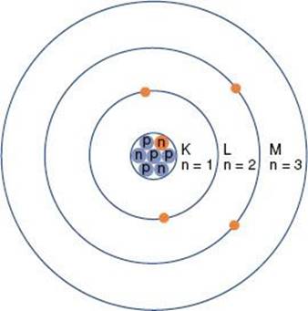
The planetary model of the atom is attributed to Niels Bohr, who in 1913 theorized that the hydrogen atom consisted of an electron orbiting around a nucleus of equal and opposite charge. He extended his theory to multielectron atoms, requiring the electrons surrounding a nucleus to be arranged in distinct, concentric shells or energy levels as shown in Figure 6.1. Energy is released when an electron moves to an orbit closer to the nucleus, and energy is required to move an electron into a higher orbit. Historically, the shells are labeled, from innermost outward, by the letters K, L, M, and so forth. There are a maximum number of electrons that can be accommodated in each shell: 2 in the first shell, 8 in the second, 18 in the third, and so on. The maximum number of electrons allowed in each shell is given by 2n², where n is an integer specific to each shell and is called the principal quantum number. Other properties of the electron also have discrete values specified by quantum numbers. These include the electron’s angular momentum as it orbits the nucleus, denoted by quantum number l (l = 0, 1,…, n – 1); its spin about its axis, denoted by s (s = ±1/2); and its magnetic moment, denoted by m_l (m_l = 0, ±1,…, ±l). Thus, each electron in an atom has an associated set of quantum numbers (n, l, s, m_l). This is the basis of the Pauli exclusion principle, which states that no two electrons can have the same set of quantum numbers within a particular atom.

Modern physics has replaced the simplistic orbiting electron model of Bohr with a complex quantum mechanical model of diffuse electron clouds that represent probability functions of the electron’s position. However, for an understanding of radiologic physics, the simple Bohr model of a nucleus composed of protons and neutrons and surrounded by orbiting electrons in distinct orbits (energy levels) is sufficient.

The atom of an element is specified by its atomic number, denoted by the symbol Z, and its mass number, denoted by the symbol A. The atomic number is equal to the number of protons in the nucleus, and the mass number is equal to the number of nucleons (protons and neutrons) in the nucleus. Hence, A minus Z is equal to the number of neutrons, denoted by the symbol N, within the nucleus. In addition, each element has an associated chemical symbol (e.g., Co for cobalt). When these definitions are used, the standard notation to specify an atom is , as illustrated by , which is a radioactive isotope of the element cobalt that has an atomic number of 27 (i.e., 27 protons) and a mass number of 60 (i.e., 60 nucleons, or 27 protons and 33 neutrons).

Isotopes of an element (e.g., , , and ) have the same atomic number but different numbers of neutrons and therefore different mass numbers. Isotopes have the same chemical properties but have different physical properties. Atoms such as and , which have the same mass number but different numbers of protons and neutrons, are called isobars. Atoms such as and , which have the same number of neutrons but different atomic and mass numbers, are called isotones.

FIGURE 6.1. Schematic drawing of the Bohr model of the atom. The nucleus contains protons (p) and neutrons (n). Electrons revolve around the nucleus in specific orbits having discrete energy levels. By convention, the orbits (energy levels) are assigned either quantum numbers (n = 1, 2, 3, …) or letters (K, L, M,…).

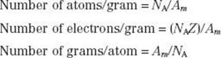
Every atom has a characteristic atomic mass A_m (sometimes referred to as atomic weight). The gram-atomic mass of an isotope is the amount of isotope in grams that is numerically equaled to the isotope’s atomic mass. For example, 1 g-atomic mass of carbon-12 is 12 g. One gram-atomic mass contains 6.0228 × 10²³ atoms, a constant that is called Avogadro’s number (N_A). Useful parameters that can be calculated using Avogadro’s number are as follows:

The closer the electrons are to the nucleus, the more tightly bound they are to the nucleus. This results from the attraction between the negatively charged electrons and the positively charged nucleus and is referred to as the Coulomb or electrostatic force. To move an electron from an inner shell to an outer shell (excitation) or to remove it completely from the atom (ionization), energy must be supplied. The energy required to remove an electron completely from an atom is called the binding energy for the electron. Binding energies are considered negative because energy must be supplied to remove the electron from its orbit. Atomic shells often are described in terms of binding energy, as shown in Figure 6.2 for the tungsten atom. The binding energies for the K, L, and M shells are –69,500, –11,000, and –2,500 eV, respectively. The electrons in the outermost shells are called valence electrons and have a binding energy of only a few electron volts because they are very loosely bound. These electrons determine the atom’s chemical properties.

FIGURE 6.2. Schematic drawing of tungsten atom showing electron configuration and energy levels. (From Johns HE, Cunningham JR. The physics of radiology, 4th ed. Springfield, IL: Charles C Thomas; 1983.)

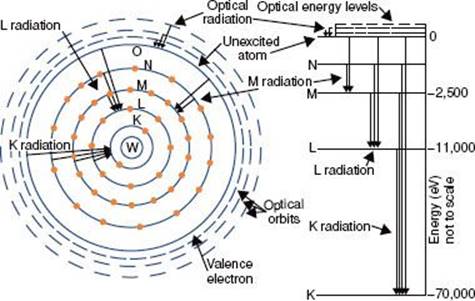
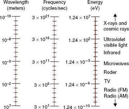
FIGURE 6.3. Electromagnetic spectrum extending over several orders of magnitude, with values of wavelength and frequency, and identifying values in some of the more common regions of the spectrum.

ELECTROMAGNETIC RADIATION

Electromagnetic radiation can be represented by a varying electric and magnetic field that is conveniently described using a sine-wave model. The sine wave is characterized by two parameters: the frequency,represented by the Greek letter v, and the wavelength, represented by the Greek letter λ. The wavelength is the distance from one crest of the sine wave to another; the frequency is the number of complete cycles or oscillations per second and is measured in hertz (Hz). The product of the frequency and wavelength is the speed with which the wave is propagated, which in a vacuum is the speed of light (c = 3 × 10⁸ m/sec).

Electromagnetic radiation wavelengths extend from approximately 10⁷ to 10⁻¹³ m. The frequencies associated with these radiations are approximately 10¹ to 10²¹ Hz. the electromagnetic spectrum shown in Figure 6.3 includes the radio and television bands; radar and microwaves; the infrared, visible, and ultraviolet regions; and x-rays and cosmic rays.

Quantum physics allows electromagnetic radiation to be represented as waves and also as particles, called photons. This is referred to as the wave–particle duality of nature. The photon energy is directly proportional to the classic wave frequency and is related to it through a constant of proportionality known as Planck’s constant (h), which has a numerical value of 6.625 × 10⁻³⁴ J-sec. The relationship between energy, E, and frequency, v, is given by the following equation:

The relationship between photon energy and photon wavelength is given by the following equation:

in which c is the speed of light in a vacuum. These relationships show that as the wavelength becomes shorter or the frequency becomes larger, the energy of the photon becomes greater.

X-RAYS

Wilhelm Conrad Röentgen discovered x-rays on November 8, 1895.⁶ He observed that a paper screen coated with fluorescent material glowed when placed in the vicinity of a tube of gas at low pressure through which electricity was being passed. We now know that the x-rays were produced where the electron beam struck the anode. Energetic electrons that impinge on matter interact with either the orbital electrons or the nuclei of target atoms. The kinetic energy of the electrons then is converted into thermal energy or electromagnetic energy (in the form of x-rays).

The impinging electron’s kinetic energy is converted into thermal energy through interaction with an outer-shell electron of a target atom, which raises it to a higher energy level (referred to as excitation). The excited electron then returns to the normal energy level with the emission of low-energy electromagnetic radiation (infrared).

If the impinging electron’s kinetic energy is high enough, the interaction can free an orbital electron (referred to as ionization), which then can result in the production of electromagnetic radiation (characteristic x-rays) when an outer orbital electron moves to the electron vacancy produced via ionization (Fig. 6.4). The characteristic x-ray energy is equal to the difference in the binding energies of the two orbital electrons involved. Occasionally, this excess energy is transferred directly to another orbital electron, causing it to be emitted from the atom. Such electrons are called Auger electrons.

The impinging electron also can lose its kinetic energy via a process called bremsstrahlung (braking radiation), which occurs when the incident electron interacts with the electric field of the nucleus (rather than the orbiting electrons) and is deflected and loses energy. This loss of energy reappears in the form of an x-ray photon. The impinging electron can lose any amount of its kinetic energy in the bremsstrahlung process. Thus, the x-radiation produced via the bremsstrahlung process is characterized by having a continuous range of energy values, unlike characteristic x-rays, which have only discrete energy values. A bremsstrahlung spectrum (i.e., a graph of x-ray intensity vs. energy) is shown in Figure 6.5. Superimposed on the continuous bremsstrahlung x-ray spectrum are the characteristic x-rays. The maximum energy of a bremsstrahlung x-ray is numerically equal to the maximum energy of the incident electrons. The direction of emission of the bremsstrahlung x-ray depends on the energy of the incident electron, with higher-energy electrons producing more-forward-directed x-rays.

FIGURE 6.4. Schematic diagram illustrating characteristic x-ray production.

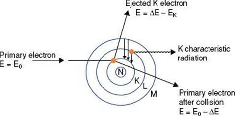
FIGURE 6.5. A bremsstrahlung x-ray spectrum calculated for a thick tungsten target extending from zero to the maximum energy of the electron. The dotted lines are for no filtration, and the solid curves are for a filtration of 1-mm aluminum. Note the superimposed characteristic x-ray emission spectrum. (From Johns HE, Cunningham JR. The physics of radiology, 4th ed. Springfield, IL: Charles C Thomas; 1983.)

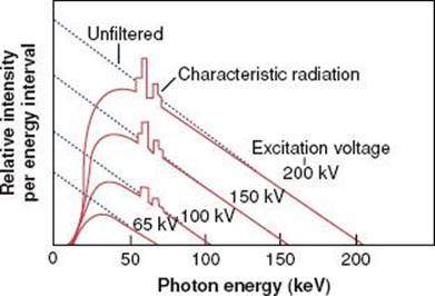
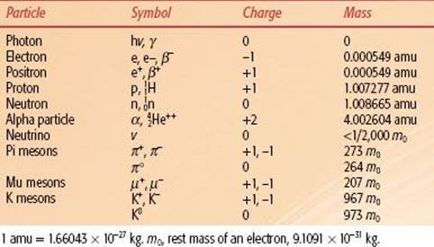
TABLE 6.1 PARTICLES OF INTEREST IN RADIATION THERAPY

RADIOACTIVITY

In 1896 Henri Becquerel conducted experiments in which he wrapped a photographic plate in black paper to keep out the light and then placed pieces of various elements against the wrapped plate.⁷ He discovered that the mineral pitchblende emitted x-rays. Other elements—such as thorium, actinium, and two new elements (polonium and radium) discovered by Pierre and Marie Curie⁸—also emitted x-rays. Further experiments showed that the radioactive elements emitted three types of radiation: α-particles, having a positive electrical charge; β-particles, having a negative charge; and high-energy γ-rays, having no charge at all. We now know that an α-particle is a helium nucleus, β-particles are electrons, and γ-rays are electromagnetic radiation that is similar to x-rays except that it originates from within the nucleus of the atom.

Many other elementary particles have since been discovered and are important topics of current physics research, but they are not germane to our discussion of radiation oncology physics. Properties of the particles relevant to radiation therapy are listed in Table 6.1.

The radioactive decay processes are related to the forces involved. Huge electrostatic (Coulomb) forces of repulsion exist between the positively charged and closely spaced protons in a nucleus. However, a nuclear force of attraction (called the strong nuclear force) exists among the neutrons and protons, binding them together to form the nucleus. The strong nuclear force is much more complicated than the electrostatic (Coulomb) force and is still not completely understood. However, it is known that the strong nuclear force between nucleons depends on the distance between them and is effective only over a very short distance, whereas the electrostatic force decreases with the square of the distance. The strong nuclear force easily overcomes the repelling electrostatic force as long as the protons are very close together. However, for a large nucleus, the strong nuclear force binding the nucleons together may be weaker on opposite sides of the nucleus than the repelling electrostatic force. Therefore, a large nucleus is not as stable as a smaller nucleus.

Because neutrons interact through the attractive strong nuclear force and not the repelling electrostatic force, they can be considered stabilizing particles for the nucleus. For example, in light nuclei, only an equal number of neutrons and protons are required, but in heavier nuclei, the number of neutrons must be about 1.5 times greater than the number of protons to counteract the repelling electrostatic forces of the protons. A nuclide having too many more protons than neutrons is said to have an unfavorable N-to-Z ratio and thus undergoes radioactive decay to reach a stable configuration.

The decay constant of a radioactive nucleus is defined as the fraction of the total number of atoms that decay per unit of time and is denoted by the symbol λ. The decay process can be represented mathematically. If N₀ radioactive nuclei are initially present in a particular sample, the number of radioactive nuclei, N, remaining at a particular time, t, is given by the following equation:

Activity, which describes the radioactivity of a sample and is denoted by the symbol A, is defined as the total number of disintegrations per unit of time interval and is given by the following relationship:

This decay-constant equation can be expressed in terms of activity:

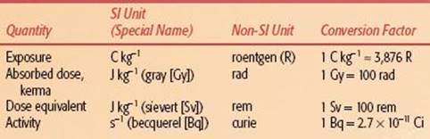
where A is the activity at time t and A₀ is the initial activity. The curie (Ci), a unit of activity, is equal to 3.7 × 10¹⁰ disintegrations per second, the approximate number of decays per second by 1 g of ²²⁶Ra. The becquerel (Bq), the special name in the International System of Units (SI) for the measure of activity, is equal to one disintegration per second (Table 6.2).

The half-life of a radioactive nuclide is the time required for the number of atoms in a particular sample to decrease by one-half. The half-life, T_1/2, is related to the decay constant by the following equation:

The average life, T_a, of a radioactive nuclide is related to the decay constant and the half-life by the following equation:

The average life represents the time period that a hypothetical source would need—if it retained its original activity for that time period and then suddenly decayed to zero activity—to produce the same number of disintegrations as produced over an infinite time period by the source if it decayed exponentially.

Gamma decay occurs when a nucleus undergoes a transition from a higher to a lower energy level. In this process, a high-energy photon, called a γ-ray, is emitted. These γ-rays are identical to the x-rays emitted by excited atoms, except that γ-rays originate from within the nucleus and x-rays originate from outside the nucleus. Half-lives for γ decay are usually very short, typically 10⁻¹⁵ second.

Closely related to γ decay is the process called internal conversion. Instead of emitting a γ-ray, the excess energy from the excited nucleus is transferred to an electron in one of the inner atomic shells, causing ejection of the electron from the atom with emission of characteristic x-rays. The probability of internal conversion occurring increases as the atomic number increases.

In β decay, a neutron within the nucleus is converted into a proton, and an electron and an antineutrino are emitted, or a proton is converted into a neutron, and a positron and a neutrino are emitted:

TABLE 6.2 INTERNATIONAL SYSTEM OF UNITS (SI UNITS) FOR RADIATION THERAPY

The positron was discovered in cosmic ray experiments in 1932. It is a positively charged particle with the same mass and spin as the electron and is considered the antiparticle of the electron. The neutrino and its antiparticle, the antineutrino, are massless particles (or at least have a very small mass) having no charge that carry opposite spins and account for the conservation of energy and continuous energy spectrum observed for β decay. Particle–antiparticle pairs interact by annihilating each other, converting all their mass into electromagnetic energy (two γ-ray photons, each of 0.51 MeV). In β decay, the emitted particles may vary in the kinetic energy they possess, which is rarely > 3MeV. Half-lives for β decay are long compared with γ decay half-lives, varying from seconds to years. The forces responsible for the β decay processes are weak compared with both the strong nuclear force and the electrostatic force among the nucleons. Accordingly, the force responsible for β decay is referred to as the weak nuclear force.

Electron capture is an alternative to positron decay. In this process, an electron, usually in the K shell, is captured within the nucleus and combined with a proton to create a neutron. Electron capture most often is followed by γdecay to release any excess nuclear energy.

Alpha decay occurs in nuclides with atomic number >82 and where the ratio of neutrons to protons is low, thus resulting in the repulsive Coulomb force of the protons overcoming the attractive strong nuclear force. The emitted α-particle is a helium nucleus (two protons and two neutrons). The kinetic energy for a particular α decay is monoenergetic (i.e., the transition may be to an excited energy state with subsequent γ emission) and often 4 to 5 MeV. Half-lives range from 10⁻³ to 10¹⁰ years. The radioactive decay of radium to radon is an example of α decay, where the Q term represents the total energy release in the transition (called transition energy). For example,

The most recent version of the periodic table of the elements shows a grouping of 118 elements (elements 117 and 118 have not yet been observed but are included to show their expected positions). Only the first 92 occur naturally; the remaining ones have been produced artificially. In general, the elements with high atomic number tend to be radioactive; in fact, all but one of the elements with atomic number >82 (lead) are radioactive; only Bi is stable.

The naturally occurring radioactive elements have been grouped into three radioactive series called the uranium series, the actinium series, and the thorium series, all of which terminate with a stable isotope of lead. The uranium series provides an example of radioactive nuclides undergoing successive transformations through α and β decay in which the parent nuclide produces a radioactive product called the daughter nuclide.

When the half-life of the parent nuclide is longer than the half-life of the daughter nuclide, an equilibrium condition exists. When this occurs, the ratio of the activity of the daughter nuclide to the activity of the parent nuclide becomes constant, and the apparent decay rate of the daughter nuclide is controlled by the parent nuclide’s decay rate. Two types of radioactive equilibrium conditions are defined: transient equilibrium and secular equilibrium.Transient equilibrium is established when the parent nuclide’s half-life is not much greater than the daughter nuclide’s half-life (Fig. 6.6). In secular equilibrium, the half-life of the parent nuclide is much greater than that of the daughter nuclide (Fig. 6.7). The two types of equilibrium are described mathematically by the following equations, in which A_P and A_D represent the activity of the parent and daughter nuclides, respectively:

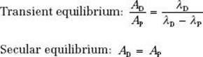
FIGURE 6.6. Transient equilibrium. Shown is a semilog plot of activity versus time for parent and daughter radionuclides illustrating conditions of transient equilibrium that may be achieved when the parent nuclide’s half-life is not much greater than the half-life of the daughter nuclide. Once equilibrium is established, the daughter activity exceeds the parent activity, and both decay with the half-life of the parent.

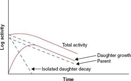
FIGURE 6.7. Secular equilibrium. Shown is a semilog plot of activity versus time for parent and daughter radionuclides illustrating conditions of secular equilibrium that may be achieved when the parent nuclide’s half-life is much greater than the half-life of the daughter nuclide. Once secular equilibrium is established, activities of both parent and daughter are equal.

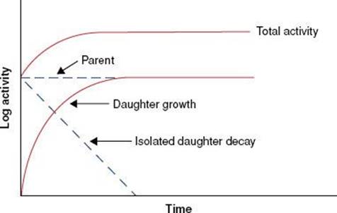
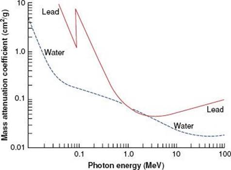
FIGURE 6.8. Mass attenuation coefficient for lead and water. Note sharp discontinuities, which are called absorption edges. (From Johns HE, Cunningham JR. The physics of radiology, 4th ed. Springfield, IL: Charles C Thomas; 1983.)

INTERACTION OF PHOTONS WITH MATTER

As stated previously, x-rays and γ-rays may be considered as bundles of energy called photons. If an x-ray photon enters a thin layer of matter, it is possible that it will pass through without interaction, or it may interact (usually with the atomic electrons, but sometimes with the atomic nuclei) in one of five different ways (coherent scattering, photoelectric effect, Compton scattering, pair production, and photodisentegration). The probability that a photon will interact when it traverses through a given thickness of material is the product of the individual interaction probabilities for each of these processes. The attenuation process can be described mathematically by the following equation:

where N₀ is the number of photons in the beam impinging on an absorber of thickness x, e is the base of the natural logarithms, and μ is the linear attenuation coefficient. The quantity μ is actually the sum of the individual attenuation coefficients for the five processes. Its numerical value depends on the energy of the photon and the type of attenuating material.

There are a variety of tabulated attenuation coefficients, including the linear attenuation coefficient (μ), the mass attenuation coefficient (μ/ρ), the mass energy-transfer coefficient (μ_t/ρ), and the mass energy-absorption coefficient(μ_en/ρ). Each type of coefficient is intended for use in the solution of different types of attenuation or energy-absorption problems; division by ρ, the physical density of the medium, makes the coefficient medium independent. Figure 6.8 shows the mass attenuation coefficient for lead and water as a function of incident photon energy. The discontinuities where the attenuation coefficient suddenly increases are called absorption edges and occur at photon energies just equal to the binding energy of a specific electron shell.

The thickness of material that reduces the number of photons transmitted to one-half the incident number is termed the half-value layer (HVL). The HVL is related to the linear attenuation coefficient by the following equation:

This parameter is used to describe the quality or penetrability of the radiation and is discussed later in this chapter.

Coherent or Classical Scattering

If the photon energy is low enough that the quantum effects of the interaction are unimportant and the bound electron(s) can be regarded as essentially “free,” the interaction corresponds to the “classical scattering” situation (called coherent scattering), in which the incident electrical field accelerates one or more orbital electrons and causes them to radiate. There are two types of coherent scattering: Thomson scattering, in which a single orbital electron is involved, and Rayleigh scattering, in which the orbital electrons act as a single group. In coherent scattering, no energy is transferred; only the direction of the incident photon is changed. The coherent mass attenuation coefficient is denoted by σ_coh/ρ.

FIGURE 6.9. Photoelectric effect. In this type of photon interaction, the incident photon disappears, and an electron is ejected with kinetic energy equal to the incident photon’s energy minus the binding energy of the electron. Characteristic x-rays and Auger electrons are emitted as the atom’s electrons cascade to fill the vacancy created by the ejected electron.

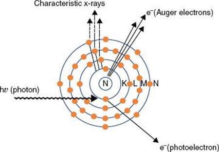
FIGURE 6.10. Compton effect. In this type of photon interaction, the incident photon interacts with one of the atom’s outer electrons, and the energy is shared between the ejected electron and a scattered photon.

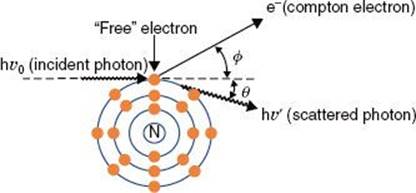
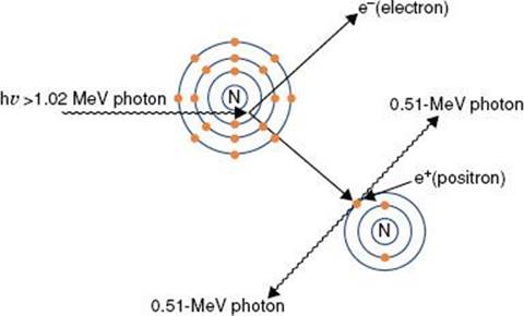
FIGURE 6.11. Pair production. In this type of photon interaction, the incident photon interacts with the electromagnetic field of the nucleus. The incident photon disappears, and two energetic electrons (a positron and a negatron) are produced. Two annihilation photons of energy 0.511 MeV then are produced when the positron interacts with its antiparticle, another electron.

Photoelectric Effect

In the photoelectric effect, the total energy of the photon is transferred to an orbital electron, usually close to the nucleus, and the photon disappears. The electron then is ejected from the atom with an energy equal to the energy of the photon minus the binding energy of the electron (Fig. 6.9). The direction in which the electron is emitted depends on the energy of the incident photon. For the low-energy photons (e.g., 50 keV) the photoelectron is ejected at a large angle with respect to the incoming photon’s direction, increasing in the forward direction as the photon’s energy increases. After ejection of the electron, the neutral atom becomes a positively charged ion with a vacancy in an inner shell that must be filled. The atom returns to a stable condition by filling the vacancy with a nearby, less tightly bound electron farther out from the nucleus, and characteristic x-rays or an Auger electron is emitted.

The probability that a given photon will interact by means of the photoelectric process (denoted by τ/ρ) is a function of both the photon’s energy and the atomic number of the target atom. For the process to occur, the incident photon must have energy greater than the binding energy of the involved orbital electron. In general, the probability per electron that a photon will undergo a photoelectric interaction is inversely proportional to the third power of the photon’s energy and directly proportional to the third power of the atomic number of the target atom.

Compton Scattering

In Compton scattering, the incident photon interacts with a loosely bound orbital electron in which part of the photon’s energy is transferred to the electron as kinetic energy and the remaining energy is carried away by another photon (Fig. 6.10). The binding energy of the electron is insignificant compared with the incident photon’s energy and thus can be ignored. The energy of the Compton-scattered photon is equal to the difference between the energy of the incident photon and the energy transferred to the electron. If the incoming photon’s energy is low (e.g., 100 keV), very little energy is transferred to the electron. As the photon’s energy increases, a greater proportion of the energy is transferred to the electron, so the scattered photon necessarily retains a smaller proportion of the incident energy. The photon may be scattered at any angle with respect to the direction of the incident photon, but the Compton electron is confined to angles between 0 and 90 deg with respect to the direction of the incident photon. If the incoming photon’s energy is low, the distribution of the scattered photons is isotropic (equal in all directions). The scatter angles decrease for photons and electrons as the incident photon’s energy increases (e.g., at megavoltage photon energies, both are scattered predominantly in the forward direction).

As a result of conservation of energy and momentum, the energies of the incident photon, hv₀, the scattered photon, hv′, and the scattered electron, E, are given by the following relationships:

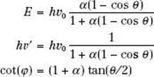
where α = hv₀/m₀c², and m₀c² is the rest energy of the electron (0.511 MeV). If hv₀ is expressed in MeV, then α = hv₀/0.511.

The probability that a photon will interact with a target atom via the Compton process (σ_c/ρ) depends on the energy of the incoming photon, generally decreasing as the energy of the photon is increased. The probability of a Compton interaction is nearly independent of the atomic number of the absorber and is directly proportional to the number of electrons per gram.

Pair Production

Pair production (Fig. 6.11) is possible only with photons having energies >1.02 MeV. When such an energetic photon approaches closely enough to the nucleus of the target atom, the incident photon energy may be converted directly into an electron–positron pair. Energy possessed by the photon in excess of 1.02 MeV appears as kinetic energy, which may be distributed in any proportion between the electron and the positron. When the positron comes to rest, it combines with an electron, and both particles then undergo mutual annihilation, with the appearance of two photons with energy of 0.511 MeV traveling in opposite directions. The probability of pair production (π/ρ) occurring increases rapidly with incident photon energy above the 1.02-MeV threshold and is proportional to Z² per atom, Z per electron, and approximately Z per gram.

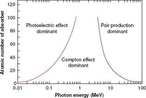
FIGURE 6.12. Relative importance of the three principal modes of interaction as a function of photon energy and atomic number of absorber. (From Hendee WR, Ritenour ER. Medical imaging physics, 3rd ed. St. Louis: Mosby-Year Book; 1992.)

Photodisintegration

In photodisintegration, a high-energy photon interacts with the nucleus of an atom, totally disrupting the nucleus, with the emission of one or more nucleons. It typically occurs at photon energies much higher than those encountered in radiation therapy. However, it is important to account for this in designing shielding around high-energy accelerators, as this interaction is a source of low-energy neutrons.

Relative Importance of Interaction Processes

Figure 6.12 illustrates the relative importance of the photoelectric, Compton, and pair-production processes—the three principal modes of interactions pertinent to radiation therapy—as a function of energy and atomic number of the absorber. For example, for an absorber with an atomic number approximately equal to that of tissue (Z = 7) and for monoenergetic photons, the photoelectric effect is the dominant interaction below about 30 keV. Above 30 keV, the Compton effect becomes dominant and remains so until approximately 24 MeV, at which point pair production becomes the dominant interaction. The total mass attenuation coefficient accounting for all the photon interactions discussed is given by the sum of the individual coefficients:

INTERACTION OF PARTICLES WITH MATTER

Electrons

An electron loses its kinetic energy when traversing matter via interactions that can be either elastic, in which no kinetic energy is lost, or inelastic, in which some portion of the kinetic energy is changed into some other form of energy. Elastic collisions occur with either atomic electrons or with atomic nuclei and are characterized by a change in direction of the incident electron with no loss of kinetic energy. Inelastic collisions can occur with atomic electrons, resulting in ionizations and excitations of atoms, or inelastic collisions with atomic nuclei, which result in the production of bremsstrahlung x-rays (radiative losses). In the case of ionization, it is possible for the ejected electron to acquire enough kinetic energy to cause additional ionizations of its own. These electrons are called secondary electrons or δrays, and they can go on to produce additional ionizations and excitations. The typical energy loss in tissue for a therapeutic electron beam, averaged over its entire range, is about 2 MeV/cm in water.

The complete description of the energy and depth of penetration of the moving electrons at any point in the medium is complicated by the fact that the electrons are very much lighter than the atomic nuclei. As a result, the electron can lose a very large fraction of its energy in a single process and thus can be deflected by very large angles. This means that even if the electron beam is monoenergetic when first impinging on a medium, there will be a large variation among all the moving electrons as to where in the medium each will stop. This is referred to as range straggling.

Protons and Light Ions

Protons traverse relatively straight paths through matter, slowing down continuously by interactions with atomic electrons and with atomic nuclei. This results in depth–dose characteristics that show an approximately constant absorbed dose value over most of the beam range until near the end of the proton’s range, where a very sharp increase in dose occurs (called the Bragg peak), as shown in Figure 6.13. Dose at the peak is approximately four times the dose at the surface, and the distal width of the peak is on the order of 1 cm, depending on beam energy and beam energy spread. Depth–dose characteristics customized for individual patients can be generated by superposition of multiple proton beams having different energies. This technique creates a spread-out Bragg peak that covers the target volume and decreases sharply to zero dose a few millimeters beyond the target. The relative biologic effectiveness (RBE) of proton beams is similar to that of other low-linear-energy transfer radiation, such as photon and electron beams. Pagnetti et al.⁹ measured RBE equal to 1.0 in the plateau region and 1.1 in the center of the Bragg peak for a 250-MeV beam. Therefore, the clinical response established for photon and electron treatments is considered applicable to proton treatments.

Neutrons

Neutrons, like photons, are uncharged and thus are an indirectly ionizing radiation, which are exponentially attenuated by matter. The interactions are through processes that are primarily nuclear. They include elastic scattering with nuclei that make up the body’s tissues (hydrogen, oxygen, carbon, nitrogen, etc.). Neutron interactions result in recoil protons and charged nuclear fragments that have relatively low energy. The RBEs of these resultant particles are not fully known, thereby complicating the understanding of the relationship between clinical response and absorbed dose.

RADIATION THERAPY TREATMENT MACHINES

Kilovoltage Units

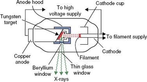
Before 1951, most radiation treatment units were kilovoltage x-ray machines capable of producing photon beams having only limited penetrability. Today, this type of machine is still used in some clinics for the treatment of skin cancer. In these machines, the electrons are accelerated by an electric field produced from a high voltage generated in a transformer that is applied directly between the filament (cathode) and the x-ray target (anode). A schematic diagram of a radiation therapy x-ray tube is shown in Figure 6.14. The potential difference (kVp) is variable on these machines, and metal filters can be added to absorb the lower-energy photons preferentially, changing the penetrability of the beam. The combination of variable kVp and different filtration provides the capability of generating multiple x-ray beams. The degree of penetrability is used to categorize the units as contact, superficial, and orthovoltage (deep-therapy) x-ray machines. A more detailed review of these type of treatment machine is provided by Biggs et al.¹⁰

FIGURE 6.13. Drawing illustrating the way in which the Bragg peak for a proton beam can be spread out. Curve A is the depth–dose distribution for the primary beam of 160-MeV protons at the Harvard cyclotron. Beams of lower intensity and shorter range, as illustrated by curves B to E, can be added to give a composite curve, S, which results in a uniform dose of >2.8 cm. (From Hall EJ. Radiobiology for the radiologist, 4th ed. Philadelphia: JB Lippincott; 1994.)

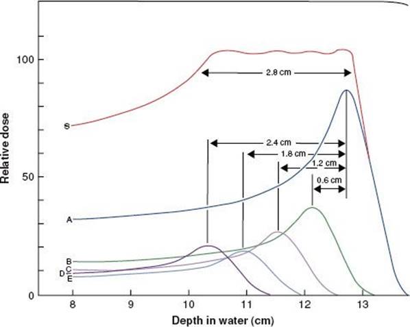
FIGURE 6.14. Schematic diagram of radiation therapy x-ray tube. (From Khan FM. The physics of radiation therapy, 3rd ed. Baltimore: Williams & Wilkins; 1994.)

Contact Units

A contact x-ray machine typically operates at potentials of 40 to 50 kVp and at a tube current of 2 to 5 milliamperes (mA). Attached cones are used for a source–skin distance (SSD) of typically 2 cm or less. Filters of 0.5- to 1.0-mm aluminum are used to give a typical HVL of 0.6-mm aluminum. The x-ray tube is rod shaped with an extremely thin mica–beryllium window, having an inherent filtration of 0.03-mm-aluminum equivalence, and the radiation is emitted axially. The primary radiation therapy application of a contact x-ray unit is for endocavitary irradiation of selected small rectal carcinomas.¹¹^,¹²

Superficial Units

A superficial unit is an x-ray machine that operates at potentials of 50 to 150 kVp and 5 to 10 mA. Added thickness of filtration (1-mm Al to 1-mm Al + 0.25-mm Cu) produces HVLs of 1.0 to 8.0 mm of aluminum. Attached cones typically are used; lead masks are used to define irregular fields. The SSD is typically 15 or 20 cm. These machines are used primarily to treat skin lesions.

Orthovoltage (Deep-Therapy) Units

Orthovoltage x-ray machines operate at potentials between 150 and 500 kV, with most operating between 200 and 300 kV, and with tube currents of 10 to 20 mA. HVLs of 1 to 4 mm of copper are common with the use of added filters, such as the Thoraeus filter, a combination of thin sheets of tin, copper, and aluminum arranged so that the highest–atomic number sheet is always closest to the x-ray target, ensuring that the higher-energy characteristic x-rays are absorbed by the lower-Z metal. Treatment fields usually are defined using detachable cones. The SSD is typically 50 cm. Very few of these types of machines are still in clinical use.

Supervoltage and Megavoltage Photon and Electron Beam Treatment Units

X-ray treatment machines operated in the range of 500 to 1,000 kV were designated as supervoltage therapy machines.¹³ The resonant transformer x-ray machine is an example of this type of kilovoltage machine. X-ray treatment machines that can produce beams 1 MV or greater have been designated as megavoltage therapy machines. One of the first megavoltage machines was the Van de Graaff generator,which operated at 1 to 2 MV. Another early type of megavoltage machine was the betatron, first developed in 1941 by Kerst.¹⁴ Betatrons used in radiation oncology produced x-ray beams with energies of >40 MV. All of these early machines are now obsolete and no longer in clinical use. Details on the history and development of these early accelerators used in radiation therapy can be found in the textbook by Karzmark et al.¹⁵

Cobalt-60 Teletherapy

The first cobalt-60 (⁶⁰Co) teletherapy machine was loaded with its ⁶⁰Co source in August 1951 in the Saskatoon Cancer Clinic, Saskatoon, Canada, and the first patient was treated on November 8 of that year.¹⁶^,¹⁷ A detailed review of ⁶⁰Co teletherapy machines is provided by Glasgow.¹⁸ The advantages of a ⁶⁰Co teletherapy machine are its relative constancy of beam output, predictability of decay because of a well-defined half-life, and lack of day-to-day small-output fluctuations typically found in electrical machines. Disadvantages include the need for source replacement approximately every 4 to 5 years, poor field flatness for large fields and large penumbra, and lower depth dose compared with high-energy photons generated by medical linear accelerators and discussed later. These types of machines became a mainstay for radiation therapy for nearly three decades but are rarely used in U.S. clinics today. Isocentric units with source-to-axis distance (SAD) of 80 or 100 cm were designed with maximum field sizes of 40 × 40 cm at the machine isocenter for the 100-cm SAD machine. Source activities vary from about 5,000 to 13,000 Ci in 1.5- to 2.0-cm-diameter sources and yield exposure rates from 150 to 250 R/min at 1 m. The radiation consists of 1.17- and 1.33-MeV γ-rays having a d_1/2 in tissue (the depth at which the dose has been reduced to 50% of the maximum dose value) of about 10 cm.

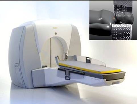
FIGURE 6.15. Elekta Gamma Knife (Elekta AB, Stockholm, Sweden) is a dedicated stereotactic radiosurgical device first developed in 1968 by Dr. Lars Leksell, a Swedish neurosurgeon, to provide highly accurate radiation ablative treatment of intracranial targets. Shown is the latest model, the Gamma Knife Perfexion, which broadens both the techniques and the scope of treatments, including the ability to treat lesions in the upper cervical spine.

Gamma Knife

A second type of treatment machine that makes use of ⁶⁰Co sources is the Elekta Gamma Knife (Elekta AB, Stockholm, Sweden), which is a dedicated stereotactic radiosurgical device that was developed in 1968 by Dr. Lars Leksell,¹⁹ a Swedish neurosurgeon. This machine made it possible to deliver a single, large dose of highly conformal radiation (γ-rays) precisely to a number of intracranial sites using multiple fixed ⁶⁰Co sources aimed at a center point. The Gamma Knife has three basic components—a spherical source housing, four collimator helmets, and a couch with electronic controls. The source housing (models U, B, and C) contains 201 ⁶⁰Co sources distributed in a quasihemispherical arrangement. The γ-rays from each source converge to the unit center point (UCP), which is 40 cm away from each source. The UCP is analogous to the isocenter of a teletherapy machine and is the location where the target volume must be positioned during a treatment. This is accomplished by the three-axis coordinate system on the Leksell stereotactic frame. Each source has an activity of approximately 30 Ci when newly installed, and the 201 sources combined provide a dose rate of approximately 300 cGy/min at the UCP. Along the path to the UCP, the radiation beam from each source is collimated twice—once by a primary collimator and then by one of four secondary collimator helmets. For each helmet, 201 tungsten collimators define specified circular apertures (4, 8, 14, or 18 mm projected at the UCP). To conform the radiation dose to the shape of the target in the patent, various combinations of aperture diameters, aperture blocking (plugging), irradiation times, and head positions are used. A specific combination of these four parameters defines what is referred to as a shot in Gamma Knife terminology. Hundreds of thousands of patients have been treated using this type of treatment machine.

More recently Elekta introduced a new model, the Gamma Knife Perfexion (Fig. 6.15), which is a major change in design from the previous models, with several advanced features, including an enlarged internal patient cavity for extended access to peripheral cranial anatomy. Unlike the earlier models, the Perfexion moves the entire patient on the couch to each stereotactic x, y, and z coordinate. The sources are arranged radially and divided into eight moving sectors with 24 sources each. Each sector is independently selectable, thereby providing various sector combinations for aperture size or blocking at each shot position during treatment. With the introduction of its associated Extend System accessory, the Perfexion has an increased reach to allow treatments to the upper cervical spine.

Linear Accelerators

The first microwave electron linear accelerator (8 MV) for medical use became operational in 1953 at the Radiation Research Center of the Medical Research Council at Hammersmith Hospital in London.²⁰ The design for an isocentric gantry mount for the accelerator first was conceived by P. Howard-Flanders.²¹ Shortly thereafter, Ginzton et al.²² at Stanford University developed a 6-MV isocentric medical linear accelerator (linac). Since then there have been continued advances in accelerator design and construction, and today medical linear accelerators account for most of the operational megavoltage treatment units in clinical use.¹⁵^,²³

Figure 6.16 is a block diagram of a high-energy, bent-beam medical linear accelerator showing the major components. The linac uses electromagnetic waves of frequencies in the S-band microwave region (2,856 megahertz [MHz]) to generate an electric field. The microwave radiation is propagated through a device called an accelerator structure, and the electrons injected into the structure are accelerated by the electric field in a straight line. The accelerator structure consists of a stack of cylindrical metal cavities having an axial hole through which the accelerated electrons pass. The accelerator structure’s electric field produced by the microwaves can be either a traveling wave or standing wave design. In a traveling wave design, the electrons travel with the electric field as the field propagates through the structure with time, somewhat in the manner of a surfboarder riding the crest of an ocean wave. In a standing wave accelerator, the reflected microwave power is used to produce a standing wave electric field. In that case, the microwave power is coupled into the accelerator structure by side-coupling cavities rather than through the accelerator structure’s axial cavity apertures.

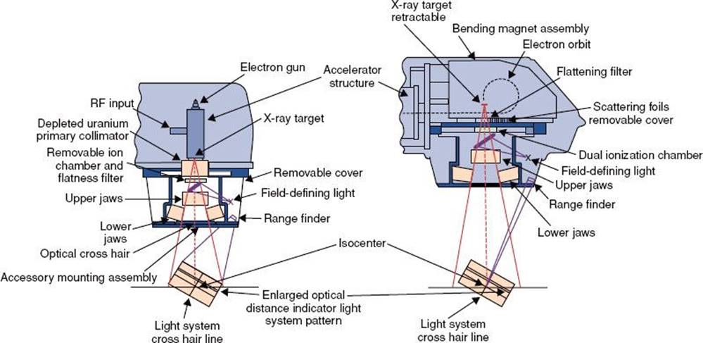
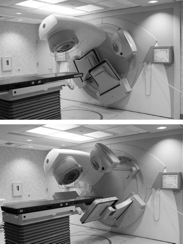
The accelerator structure in low-energy (4 to 6 MV) linacs most often is mounted vertically in the treatment head collinear along with the components associated with producing, controlling, and monitoring the x-ray beam (Fig. 6.17, left). High-energy (15 to 18 MV) linacs use a horizontally mounted accelerator structure with a beam-bending magnet system (Fig. 6.17, right). Accelerator structure technology now makes possible multiple high–dose rate photon beams of widely separated energies.

FIGURE 6.16. Schematic block diagram showing major components of a high-energy bent-beam medical linear accelerator. (Courtesy of Varian Associates, Palo Alto, CA.)

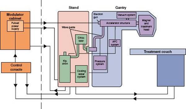
FIGURE 6.17. Schematic cutaway diagram of treatment heads for low-energy, straight-beam (left) and high-energy, bent-beam (right) medical linear accelerators. (Courtesy of Varian Associates, Palo Alto, CA.)

Other important components of a linac are the modulator, microwave power sources, electron gun, and the beam-handling components. The modulator is the source of pulsed direct current (DC) power, which is needed for the production of microwave power. Pulsed DC power is also supplied to the electron gun (a hot-wire filament that serves as the source of the accelerated electrons). The electrons are bunched before acceleration by a device called a buncher. The electron beam thus consists of pulses of bunched electrons in the form of a narrow pencil beam. The magnetron is a device that serves both as the source of the microwaves and as a power amplifier. The klystron is a device used to amplify the microwave power that is generated from a separate microwave source (RF driver). The microwave power coming from the magnetron or klystron is transported to the accelerator structure by a metallic pipe called a waveguide. A device called the circulator is used to isolate the klystron/magnetron from the reflected microwave power.

Other important components in a linac are located in the treatment head. These include the x-ray target, fixed primary collimator, scattering foils, flattening filter, monitor ion chamber, movable secondary collimator jaws, light field localizer, and optical distance indicator. In addition, the treatment head contains a significant amount of shielding material to minimize leakage radiation.

At the exit window of the accelerator structure, the high-energy electrons emerge in the form of a pencil beam of about 2 to 3 mm in diameter. In a low-energy (4 to 6 MeV) linac, the accelerated electrons proceed in a straight line and strike an x-ray target when in photon mode, producing bremsstrahlung x-rays. In high-energy linacs, because the accelerator structure is much longer and is placed horizontally or at some angle with respect to the horizontal, the electrons must be bent through a suitable angle, usually 90 or 270 deg between the accelerator structure and the target. This is enabled by the beam transport system, which consists of an achromatic focusing and bending magnet, as well as steering and focusing coils.

The primary collimator is a fixed collimator located just below the x-ray target and is used to collimate the x-ray beam in the direction of the patient treatment and reduces the leakage radiation from the x-ray source. The angular distribution of the bremsstrahlung x-rays produced by megavoltage electrons incident on a target is forward peaked. To make the x-ray beam intensity uniform across the field, a conical metal flattening filter is inserted in the beam. Filters are constructed of lead, tungsten, uranium, steel, and aluminum (or some combination of these), depending on x-ray energy. The flattened x-ray beam then passes through a monitor ionization chamber. In most cases, this system consists of several transmission-type parallel-plate ionization chambers, which cover the entire beam. These ion chambers are used to monitor the field symmetry, dose rate, and integrated dose per monitor unit.

FIGURE 6.18. Schematic illustrating the geometry of a multileaf collimator for Varian linear accelerators. The x-direction is the field width across each leaf pair, and the y-direction is the field length. (Courtesy of Varian Associates, Palo Alto, CA.)

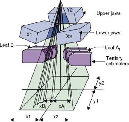
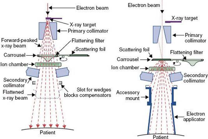
FIGURE 6.19. Schematic diagram of beam subsystems for x-ray beam (A) and electron beam therapy (B). (From Karzmark CJ, Morton RJ. A primer on theory and operation of linear accelerators in radiation therapy. Rockville, MD: Department of Health and Human Services, Public Health Service, Food and Drug Administration, Bureau of Radiological Health; 1997.)

After passing through the monitor chamber, the beam can be further collimated by continuously movable x-ray collimators, consisting of two pairs of lead or tungsten jaws, which provide rectangular field sizes ranging from 0 to typically 40 × 40 cm at a distance of 100 cm. The field size is defined by a light localizer and a mirror assembly. Independent jaw capability is now common. This flexibility allows simplified patient positioning and improved safety by avoiding overlapping field abutments without the necessity of using heavy beam-splitting blocks.²⁴ Independent jaw technology in conjunction with computer control of the dose rate can be used to create a wedge-shaped isodose pattern.²⁵

Most modern medical accelerators now come with multileaf collimator (MLC) systems (Fig. 6.18).²⁶^,²⁷ The leaf settings for each field are computer controlled. Modern treatment planning systems have the ability to configure MLC shaped fields, and the patient’s MLC configuration files are sent via a local area network to the linac’s MLC computer. Most important, computer-controlled MLC systems are used to create optimized modulated beam fluence. This form of therapy is referred to as intensity-modulated radiation therapy (IMRT) and is delivered at fixed gantry angles by (a) delivering multiple field segments (called segmental MLC [SMLC] or step-and-shoot IMRT) or (b) having the leaf pairs move across the field at a varying rate with the x-ray beam on (called dynamic MLC [DMLC] or sliding window IMRT).²⁸

In the electron mode, the accelerator’s beam current is reduced 1,000-fold and the x-ray target is retracted. An electron-scattering foil is moved into place on the beam centerline so that the accelerated pencil electron beam strikes it in order to broaden the beam and produce a flat field across the treatment field. The scattering foil typically consists of dual lead foils. The thickness of the first foil ensures that most of the electrons are scattered with only a minimum of bremsstrahlung x-rays. The second foil is generally thicker in the central region and is used to flatten the field. The bremsstrahlung produced appears as x-ray contamination of the electron beam and is usually <5% of the maximum dose. An electron applicator is mounted below the movable collimator jaws to provide the final field collimation. A schematic diagram of all the treatment head subsystems for both x-ray and electron beams is shown in Figure 6.19.

More recently, conventional medical linacs have integrated advanced imaging systems having cone beam computed tomography (CBCT) capability. Such linacs are referred to as image-guided radiation therapy (IGRT) linacs. The first commercial CBCT IGRT linac was the Elekta Synergy (Elekta).²⁹^,³⁰ The other medical linac manufacturers have also embraced the IGRT concept and have produced their own version of an IGRT linac—for example, Varian Trilogy and TrueBeam (Varian Medical Systems, Palo Alto, CA) and Siemens ARTÍSTE (Siemens Medical Solutions USA, Malvern, PA). The Synergy IGRT system (referred to as XVI) consists of a retractable kilovolt x-ray source, an amorphous silicon flat-panel imager mounted on the linear accelerator perpendicular to the radiation beam direction, and a software module for processing the data and tools for registering the images (Fig. 6.20). The XVI system provides for planar, motion, and volumetric imaging capabilities. Registration software is provided to compare the daily patient setup image with the stored prescription computed tomography (CT)–planning image, after which table adjustments can be made prior to treating the patient.

More recently, manufacturers of medical linacs and their associated planning systems have introduced features that provide rotational IMRT capability—for example, Elekta VMAT³¹ and Varian RapidArc.³² The linac-based rotational IMRT concept was first proposed by Yu³³^,³⁴ and called intensity modulated arc therapy (IMAT), but planning software was not commercially available at that time. Rotational IMRT approaches on conventional linacs may provide even more conformal dose distributions delivered in a shorter treatment time compared with SMLC- or DMLC-IMRT approaches that use only a limited number of gantry directions. In addition, plan optimization is simpler since it eliminates the planner’s iterative choices of beam number and direction. The conventional MLC approach for rotational IMRT is likely to improve IMRT plan quality and delivery efficiency,³² although this remains somewhat controversial,³⁵^,³⁶ and more users will need to report their rotational IMRT experiences over the next few years.

Microtrons

The microtron, whose concept is credited to Veksler,³⁷ is an electron accelerator that combines the basic principles of the electron linear accelerator and the cyclotron. By using magnets to recirculate the electron beam through a microwave accelerator cavity (or cavities) one or more times, it is possible to achieve a high beam energy with a low-energy accelerating section. After each orbit in the magnet, the electron bunch must arrive in phase with the accelerator microwave field. Thus, the magnet system acts as an energy spectrometer, limiting the electron energy acceptance to a narrow energy width and consequently limiting to some extent the beam current.

This concept was developed further by Schwinger,³⁸ who proposed the racetrack microtron. It uses two D-shaped magnet pole pieces that are separated by a fixed distance, between which is a linac accelerator structure. A 50-MeV unit was developed for radiation therapy applications by the Swedish firm Scanditronics (Uppsala, Sweden) and was one of the first modern intensity-modulated radiation therapy delivery systems described in the literature.³⁹ Only two of this type of microtron were installed in the United States, and both have been replaced.

FIGURE 6.20. Elekta Synergy installed at the University of California, Davis. The unit consists of a conventional multimodality medical linac with a retractable kilovolt x-ray source, an amorphous silicon flat-panel imager mounted on the linear accelerator perpendicular to the radiation beam direction, and a software module (referred to as the XVI system). Top: The x-ray source, with the amorphous silicon flat panels retracted. Bottom: With the panels extended.

Tomotherapy

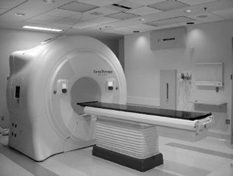
Helical tomotherapy was first proposed by Mackie et al.⁴⁰ and is now commercially available as the TomoTherapy HI-ART system (Accuray, Madison, WI).⁴¹ A short, in-line, 6-MV linac (Siemens Oncology Systems, Concord, CA) rotates on a ring gantry at a source–axis distance of 85 cm. Figure 6.21 shows the unit installed at the University of California, Davis. The intensity-modulated radiation therapy treatment is delivered while the patient-support couch is translated in the y-direction (toward the gantry) through the gantry bore in the same way as a helical CT study is conducted. Thus, in the patient’s reference frame, the treatment beam is angled inward along a helix, with the midpoint of the fan beam passing through the center of the bore. Similar to helical CT, the treatment beam pitch is defined as the distance traveled by the couch per gantry rotation divided by the field width in the y-direction (typically between 0.2 and 0.5). The width of the beam in the y-direction is defined by a pair of jaws that is fixed for any particular patient treatment to one of three selectable values (1, 2.5, or 5 cm). Laterally, the treatment beam is modulated by a 64-leaf binary MLC, whose leaves transition rapidly between open and closed states. Each leaf has a projected width of 6.25 mm at the bore center, for a maximum possible open lateral field length of 40 cm. Intensity modulation is accomplished by varying the fraction of time different leaves are opened. The individual modulation pattern can change with angle (divided into exactly 51 projections over a full revolution). During the treatment, the gantry rotates at a constant velocity with a period ranging between 10 and 60 seconds/rotation. The extent to which a treatment beam projection is modulated is characterized through what is called the modulation factor, defined as the ratio of the maximum leaf open time to the average leaf open time for the projection. Pitch and maximum permissible modulation factor are new parameters that need to be specified by the treatment planner. Highly modulated treatments achieve greater conformality but inevitably take longer to deliver. A helical MVCT image is acquired using the on-board xenon CT detector system and the 6-MV linac (detuned to 3.6 MV) with the leave fully opened when the patient-support couch is translated in the y-direction through the gantry bore. Registration software is provided to compare the daily patient setup image with the stored prescription CT planning image.

FIGURE 6.21. TomoTherapy HI-ART system installed at the University of California, Davis. A short, in-line 6-MV linac rotates on a ring gantry. Intensity-modulated radiation therapy treatment is delivered while the patient-support couch is translated through the gantry bore in the same way as a helical computed tomography study is conducted. The width of the beam in the patient-translated direction is defined by a pair of jaws that is fixed for any particular patient treatment, and laterally the treatment beam is modulated by a 64-leaf binary multileaf collimator.

CyberKnife

The use of a small X-band (~10,000 MHz) linear accelerator mounted on an industrial robotic arm was first developed for radiosurgery.⁴²^,⁴³ The robotic arm provides the capability for aiming a narrowly collimated x-ray beam with any orientation relative to the target volume. The system uses two ceiling-mounted diagnostic x-ray sources and amorphous silicon image detectors mounted flush to the floor. The treatment is specified by the trajectory of the robot and by the number of monitor units delivered at each robotic orientation. During the patient’s treatment, the CyberKnife system correlates live radiographic images with preoperative CT or magnetic resonance imaging (MRI) scans in real time to determine patient and tumor position repeatedly over the course of treatment.

New and Evolving Photon Treatment Machines

There are several other new photon beam treatment machine designs that show significant promise. For example, the four-dimensional IGRT system proposed by Kamino et al. has a unique, gimbaled x-ray head design that allows the linear accelerator head to be pivoted.⁴⁴ By easily allowing noncoplanar beams without couch rotations, new degrees of freedom are made available for IMRT optimization, and even more conformal dose distributions may be possible.

The Vero (Brainlab AG, Feldkirchen, Germany) for stereotactic radiosurgery/stereotactic body radiotherapy was recently introduced, which uses a rotating ring gantry to which a megavolt x-ray treatment head is mounted on orthogonal gimbals.⁴⁵ Image guidance systems include an electronic portal imaging device (EPID) and two fixed kilovolt x-ray tubes combined with two fixed flat-panel detectors. This dual imaging system provides planar images, CBCT, and real-time fluoroscopic monitoring.

Another highly promising IG-IMRT delivery system on the horizon, which has significant potential to improve the ability to localize and track soft tissue tumors, is the Renaissance System 1000 (ViewRay, Cleveland, OH). This device utilizes a multiheaded ⁶⁰Co rotational IMRT system with MR image guidance and has the ability to image continually during treatment even while the beam is on. In addition to the Renaissance, research continues in the development of a MRI-linac hybrid system.⁴⁶

Several investigators have also pointed out the utility of very high energy (VHE) electron beams (150 to 250 MeV).⁴⁷^,⁴⁸ Such high-energy beams are not yet available, and so only beam simulation software has been used to demonstrate the use of multi-VHE beams from opposed directions and the ability to modulated VHE beam intensity.⁴⁷^,⁴⁸ Such machines are clearly some time away, but these early studies show promise.

Proton, Light-Ion, and Neutron Beam Treatment Units

The first use of proton beams for radiation therapy is credited to Wilson,⁴⁹ who in 1946 pointed out the superior depth–dose characteristics provided by protons. Details on the history and development of proton beam radiation therapy (PBRT) machines are provided by Breuer and Smith⁵⁰ and Delaney and Kooy.⁵¹ PBRT is seeing increasing interest worldwide because its depth–dose characteristics show advantages over those of photon beams.⁵²

In most existing or proposed proton and light-ion particle treatment facilities, either a cyclotron or a synchrotron is used to accelerate proton beams to sufficient energy (200 to 250 MeV) and beam intensity.

Cyclotron

The cyclotron (Fig. 6.22) was invented by Ernest Lawrence of the University of California in 1929. It accelerates charged particles such as protons, deuterons, and light ions using a high-frequency, alternating voltage (potential difference) applied across two conducting D-shaped evacuated half-cylinders (Ds). A fixed magnetic field, perpendicular to the top of the two Ds, forces the charged particles to travel in a circular path. The charged particles accelerate only when passing through the gap between the two Ds. The beam spirals out to the edge of the container as the particle speeds increase. At this point, the particle speed approaches the speed of light. Proton beam energies of 200 to 250 MeV are considered adequate for most radiation therapy applications. Beam intensity from the accelerator must be adequate to overcome losses in the beam delivery system and provide tolerable treatment times.

FIGURE 6.22. Schematic drawing showing principles of cyclotron operation. This machine is used for accelerating positive ions and is used clinically to produce proton and neutron beams. Metal half-disks (Ds) have an evacuated center through which the protons can travel. The protons are accelerated by an oscillating electric field operating between the half-disks. A magnetic field perpendicular to the plane of the half-disks confines the charged particles in the half-disks.

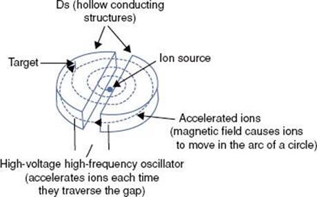
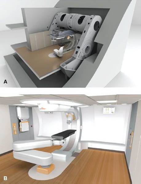
FIGURE 6.23. Rendering of next-generation proton therapy system (MEVION S250 Proton Therapy System, Mevion Medical Systems, Littleton, MA; formerly Still River Systems). (A) Outer gantry holds the proton accelerator in the center, pointing directly to the isocenter. Accelerator is a 250-MeV cyclotron specifically designed (uses superconducting magnets) for proton therapy (with intensity-modulated proton therapy capabilities, high dose rate, high reliability, and easy maintenance). (B) Treatment room depicting inner gantry and six-degree-of-freedom robotic couch.

Synchrocyclotron and Synchrotron

A synchrocyclotron varies either the magnetic field or the frequency of the applied electric field; a synchrotron varies both. By increasing these parameters appropriately as the particles gain energy, one can hold their path constant as they are accelerated. This allows the vacuum container for the particles to be a large, thin torus. In reality it is easier to use some straight sections and some bent sections using multiple bend magnets, thus creating the shape of a rounded-corner polygon. The proton beam facility at Loma Linda University Medical Center (Loma Linda, CA) is an example of this type of accelerator.⁵³

The synchrotron has the advantage of simple energy variability, whereas the cyclotron produces continuous beams with a fixed energy and higher beam intensity, making their design somewhat simpler. Beam-spreading mechanisms obtain suitable field sizes for radiation therapy by passive modulation (scattering foil) systems or by dynamic pencil-beam spot-scanning systems,⁵³ which allow dose conformation not only at the distal edge of the tumor, but also at the proximal edge. Hall⁵⁴ pointed out that there is significant neutron leakage radiation for proton treatment machines that use a scattering foil and recommended moving to the pencil-beam scanning systems.

There are at least 9 modern PBRT facilities specifically designed for radiation therapy already operating in the United States and approximately 10 more either in development or scheduled to open over the next few years.

There are only a few active clinical facilities for light-ion radiation therapy (primarily carbon ion).⁵²^,⁵⁵ Two are operational in Japan, with a third coming on line soon and a fourth soon to begin construction. Heidelberg, Germany, has the first clinical center with multiple-ion capabilities from protons to carbon, including the first gantry for carbon beams; two more are currently under construction in Germany. The Centro Nazionale di Adroterapia Oncologica (National Center for Oncological Hadrontherapy) in Pavia, Italy, was scheduled to begin treatments in 2011. In addition, facilities are under construction in France and Austria.

Light-ion radiation therapy requires beams at much higher energies than proton therapy. For example, a proton beam of 150 MeV can penetrate 16 cm in water. To achieve the same penetration with carbon ions, energy of 3,000 MeV or 250 MeV/per nucleon is needed. Synchrotrons are the only available sources for such high-energy ion beams, and they are large, complex machines requiring large facilities and similarly large capital expenditures.

Interest in light-ion radiation therapy is due to its combination of two important physical advantages: (a) its depth–dose characteristics and (b) high linear energy transfer (LET) in the Bragg peak region of the beam. For its depth characteristics, the ratio of the Bragg peak dose to the entrance region dose is even larger than for protons. In addition, unlike proton beam therapy, there is a large increase in the radiation LET in the Bragg peak region of the beam. The combination of these two characteristics results in a potentially unique advantage—a high LET region that can be closely conformed to the target volume.

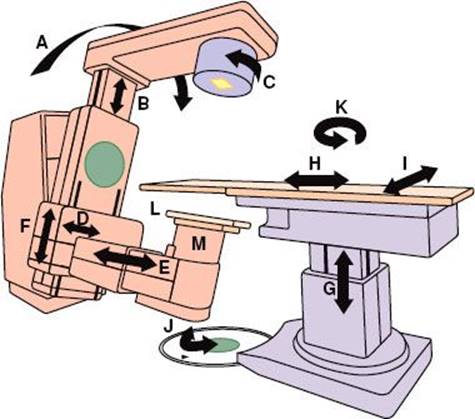
FIGURE 6.24. The basic components and motions of a radiation therapy simulator: A: Gantry rotation. B: Source–axis distance. C: Collimator rotation. D: Image intensifier (lateral). E: Image intensifier (longitudinal). F: Image intensifier (radial). G: Patient table (vertical). H:Patient table (longitudinal). I:Patient table (lateral). J: Patient table rotation about isocenter. K: Patient table rotation about pedestal. L: Film cassette. M: Image intensifier. Motions not shown include field-size delineation, radiation beam diaphragms, and source–tray distance. (From Van Dyk J, Mah K. Simulators and CT scanners. In: Williams JR, Thwaites DI, eds. Radiotherapy physics. New York: Oxford Medical Publications; 1993.)

New and Evolving Proton Treatment Machines

New technologies for the delivery of PBRT are emerging. Single-gantry systems are being designed and manufactured, including the MEVION S250 Proton Therapy System (Mevion Medical Systems, Littleton, MA; formerly Still River Systems) shown in Figure 6.23. This system uses a superconducting synchrocyclotron that is gantry mounted and incorporates image-guidance and robotic patient positioning. The first unit was scheduled to be installed at Washington University (St. Louis, MO) in late 2011.

In addition, Varian recently announced their single-room PBRT system, which uses superconducting cyclotron technology and can be expanded into a multiroom facility when needed.

A more futuristic design concept has been reported by Caporaso et al.⁵⁶ This system is being codeveloped by Compact Particle Acceleration Corp (Livermore, CA) and TomoTherapy (Madison, WI). The design is based on dielectric wall accelerator (DWA) technology (under development by the Lawrence Livermore National Laboratory, Livermore, CA⁵⁶). The goal is to make a PBRT linac so compact that it can be installed in a conventional linac treatment room. This will require an average accelerating gradient of approximately 100 MV/m to yield a linac on the order of 2 m in length. If successful, the DWA PBRT machine would produce a 200-MeV proton beam composed of individual pulses that could be varied in intensity, energy, and spot width. While the DWA is still largely at a research level of development, the realization of a compact, image-guided PBRT system that can provide rotational intensity-modulated proton therapy and be sited in a treatment room not much larger than for a conventional linac would likely be a real “game changer” for radiation therapy.

Neutron Therapy Treatment Machines

Modern neutron therapy machines use cyclotrons to accelerate protons or deuterons to energies of about 50 MeV to produce neutron beams with depth–dose characteristics equivalent to those of about 6-MV x-rays. The p,Be (protons accelerated to strike a beryllium target) reaction is used most commonly because protons are much easier to bend around the gantry of an isocentric unit, and thus the cyclotron can be much smaller and thus less expensive. The only exception is the superconducting cyclotron installed at Harper Hospital (Detroit, MI), which uses the d,Be (deuterions strike beryllium target) reaction.⁵⁷ With superconducting technology, the entire cyclotron is small enough to be rotated around the patient on isocentric rings, thus eliminating the need for bending the deuteron beam around a rotating gantry. In addition, the neutron yield for the d,Be reaction is about five times that for the p,Be reaction. More details on the history and development of neutron beam therapy machines are provided in the review by Maughan and Yudelev.⁵⁸

SIMULATORS

Conventional Simulator

Details on the development of the radiation therapy simulator and the selection, acceptance testing, and quality assurance of conventional radiation therapy simulators are provided in the review article by Van Dyk and Munro.⁵⁹ The conventional simulator mimics the functions and allowed motions of a therapy unit and uses a diagnostic x-ray tube to simulate the radiation properties of the treatment beam (Fig. 6.24). A simulator allows the beam direction and the treatment fields to be determined to encompass the projection of the target volume. Radiographic visualization of internal structures in relation to external landmarks allows special shielding devices (Cerrobend blocks) to be constructed to help minimize the dose to normal critical structures. Gantry arms are rigid enough to support heavy shielding blocks and simulated electron cones. Couch widths are similar to therapy-unit couch widths, and operating consoles feature digital displays of parameters and programmable settings for source-to-axis distance, gantry angles, and field sizes. Older models of conventional simulators were equipped with an x-ray fluoroscopy system consisting of an image intensifier and video camera system to expedite field setup and beam angulations. Modern simulator design has replace the image intensifier with amorphous silicon technology. The new imagers produce high spatial- and contrast-resolution images that approach film quality, facilitating the concept of filmless radiation oncology departments, and provide CBCT capability. While this feature allows volumetric imaging on a conventional simulator, they are still rapidly being replaced with CT simulators.

CT Simulators

In the 1980s and early 1990s, research led to the integration of a diagnostic CT scanner with what was essentially a three-dimensional (3D) treatment-planning system, which led to the concept of virtual simulation.⁶⁰^–⁶² Such a system is now referred to as a CT simulator and consists of a CT scanner, a flat-tabletop patient position–alignment system, including an orthogonal laser system, and a digital interface (DICOM) to a planning system that is equipped with virtual simulation software (Fig. 6.25). Simulation software provides many advanced image manipulation and viewing features, including beam’s-eye viewdisplay, which allows the anatomy to be viewed from the perspective of the radiation beams and allows field shaping to be done electronically at the graphics display station, and the generation of digitally reconstructed radiographs. Modern CT simulation systems incorporate large-bore CT scanners especially designed for radiation oncology, with multislice capability, high-quality laser patient positioning/marking systems, and sophisticated virtual simulation software features. Details of the virtual simulation process are discussed in some detail in Chapter 9. More details on CT simulation can be found in the review article by Van Dyk and Taylor⁶³ and articles by Mutic et al.⁶⁴^,⁶⁵

New and Evolving Simulation Machines

The most significant development now occurring with simulators is the continued integration of functional imaging with anatomic imaging in the simulation/planning process. Already commercially available are a magnetic resonance simulator and a large-bore positron emission tomography CT simulator, both with features specifically designed for radiation oncology. While not yet common in radiation oncology departments, it is very likely that multimodality imaging simulation systems will become common within the next decade and include full four-dimensional capabilities to address cases involving significant internal motion.

QUALITY OF RADIATION

The penetrability of an x-ray beam, referred to as the quality of the beam, is completely specified by its spectral distribution curve (i.e., the relative intensities of photons of various energies), which is the result of fluctuations of tube potential, the bremsstrahlung radiation process, characteristic radiation, and multiple interactions of the incident electrons and the x-ray target. The distribution of the photon energies, including the peak photon energy, in the continuous spectrum is governed solely by the x-ray tube potential. However, the energy of the characteristic photons increases with increasing atomic number of the target element. All other factors being equal, the radiation intensity is proportional to the atomic number of the target element.

Spectral distribution of an x-ray beam can be modified by placing absorbing materials of various thicknesses (i.e., filters) in the beam. In general, a filter removes relatively more low-energy photons than high-energy photons, although photons of all energies are removed to some extent. For radiation in the orthovoltage region (except for the absorption edge effect), the lower the energy of the photons, the larger is the total mass attenuation coefficient and therefore the greater is the likelihood that the photon will be absorbed. Thus, the beam emerges from the filter with a larger percentage of high-energy photons than it had on entering the filter. The beam has a greater penetration power and is said to have been “hardened” by the filter. The quality of an x-ray beam improves with increasing tube potential and with increasing thickness and atomic number of the filter.

FIGURE 6.25. Typical computed tomography simulation suite showing the scanner, flat tabletop, orthogonal laser system, virtual simulation workstation, and hardcopy output device.

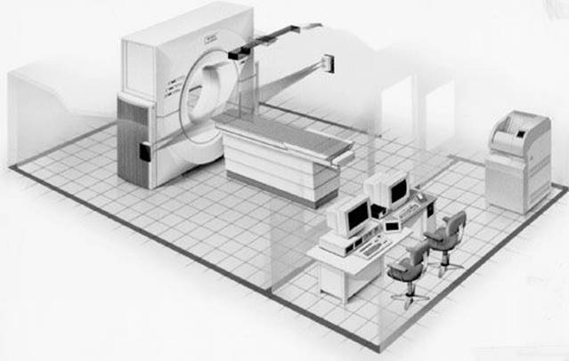
A specification of beam quality based entirely on a spectral distribution is too cumbersome for radiation therapy. The usual method of specifying beam quality in superficial and orthovoltage therapy is to list the HVL and the accelerating potential. For megavoltage beams, only the maximum energy of the electrons striking the x-ray target typically is used. The homogeneity coefficient denotes how homogeneous an x-ray beam is with respect to its photon energies. It is defined as the ratio of the first HVL to the second HVL. As the filtration is increased, the exposure rate decreases; therefore, there is a practical limit of filter thickness in orthovoltage therapy with a given combination of kilovolts, milliamperes, and treatment distance. In certain situations, it is convenient to express the quality of the x-ray beam in terms of an “equivalent energy,” which can be derived from knowledge of the HVL. The type of x-ray beam that is used in radiation therapy is always heterogeneous; however, the x-ray beam can be considered to have an equivalent energy of a monoenergetic x-ray beam that has a HVL equal to the measured HVL of the heterogeneous beam.

RADIATION EXPOSURE

In 1928 at the Second International Congress of Radiology, the ionization of air, called exposure, was adopted as the measurable effect of radiation of a photon beam.⁶⁶ As the beam passes through a material, it creates ion pairs via the ionization process. In air, these ion pairs have some mobility and can be collected by applying an electric field across the air. The number of ion pairs collected is a measure of the quantity of radiation passing through the air.

The roentgen (R), the unit for exposure, also was defined at the 1928 Congress. The definition has been modified slightly by subsequent congresses, but the basic concept remains the same. The roentgen is that amount of x- or γ-radiation that causes the associated corpuscular emission per 0.001293 g of air to produce, in air, ions carrying one electrostatic unit of charge of either sign. The value 0.001293 g is the mass of 1 cm³ of air at 0°C and 760 mm Hg pressure; “associated corpuscular emission” refers to the Compton and pair-production electrons set in motion by the interactions between the incident photons and the air molecules. By conversion of units, the roentgen can be expressed as follows:

With the advent of SI units, the roentgen no longer is used as a special name for a radiation unit, and the SI unit for exposure is coulombs per kilogram (C/kg), which is equivalent to approximately 3,876 R (Table 6.2).

The condition of electronic equilibrium must exist for the definition of the roentgen to be satisfied (Fig. 6.26). According to the definition, the electrons produced in a specified volume must spend all of their energies by ionization in air, and the total charge must be measured. However, because some electrons produced inside the specified volume create ion pairs outside the volume and some electrons produced outside the volume contribute ionization inside the specified volume, the gain and loss of ion pairs must be the same for the definition of the roentgen to be satisfied.

The free-air ionization chamber is used to measure exposure directly in roentgens.¹ It is designed to collect all the ions produced in a defined volume by the radiation beam and is used primarily by standards laboratories. Free-air chambers are bulky and too complicated to use for routine measurements. Instead, small ionization chambers called thimble chambers are typically used to measure exposure. The chamber gives a measure of the ionization produced, which then is converted to exposure in roentgens by use of an exposure calibration factor, N_x, traceable to the National Institute of Standards and Technology (Gaithersburg, MD). Thimble chambers are designed for use at specific energies; the thickness of the chamber wall is equal to the maximum electron range (electronic equilibrium established). If they are used at higher energies, at which the electron range is greater, an added wall thickness or buildup cap must be used.

FIGURE 6.26. Schematic illustrating electronic equilibrium. (From Khan FM. The physics of radiation therapy, 3rd ed. Baltimore: Williams & Wilkins; 1994.)

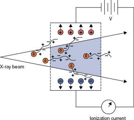
To determine the exposure rate from an x-ray or γ-ray machine, an exposure-calibrated thimble chamber (with appropriate wall thickness) and connected to an electrometer is placed at beam center, in air, at right angles to the beam’s central axis and at the point where the exposure rate is to be specified. The field size for which the exposure rate is to be measured is set, and the radiation machine is turned on for a specified time, T, to achieve a reading, M,on the connected electrometer. The reading is corrected for temperature and atmospheric pressure, timer error, stem effect, and ion-recombination effects. The therapy machine exposure rate, , is given in roentgens per minute by the following equation:

where M is the raw ionization chamber reading, N_x is the exposure calibration factor obtained from a standards laboratory, C_tp is the temperature and pressure correction factor, C_st is the stem effect correction factor, C_s is the ion-recombination correction factor, T is timer (minutes) or monitor unit setting, and α is the timer error. The temperature-pressure correction factor C_tp is given by the following equation:

The timer error α is given by the following equation:

where M₁ is the instrument reading for a single long exposure of T, M₂ is the instrument reading for n short exposures of total time T, and α is the timer error (monitor end effect for linacs) for a single exposure.⁶⁷

Beyond 3 MeV, the roentgen cannot be measured accurately, and thus calibrations of radiation therapy machines at these higher energies are performed using an exposure-calibrated ionization chamber such as a Bragg–Gray cavity, and the ionization readings are converted to absorbed dose as discussed in the following section.

ABSORBED DOSE

In 1953 the International Commission on Radiological Units and Measurements introduced the concept of absorbed dose and defined its unit, the rad.⁶⁶ Before its definition can be presented, the reader must understand the concept of dose absorption. As a beam of radiation passes through an absorbing medium, it interacts with it in a two-stage process. The first step occurs when energy carried by the photons—the indirectly ionizing particles—is transformed into kinetic energy of high-speed electrons; the second step occurs as these electrons—the directly ionizing particles—are slowed down and deposit their energy in the medium.

Kerma, an acronym for “kinetic energy released in the medium,” represents the transfer of energy from the photons to the directly ionizing particles (step 1). The subsequent transfer of energy from the directly ionizing particles to the medium (step 2) is represented by the absorbed dose and is defined in terms of the energy deposited by the radiation beam as it passes through the medium. The relationship between kerma and absorbed dose is illustrated in Figure 6.27.

The rad represents the absorption of 0.01 J/kg of the absorbing material (1 rad = 0.01 J/kg). The rad now has been replaced with the SI unit for absorbed dose (1 J/kg) given the special name of gray (Gy) (Table 6.2). By conversion of units, the gray can be expressed as follows:

FIGURE 6.27. Graphs showing schematic relationship of kerma and absorbed dose. (From Johns HE, Cunningham JR. The physics of radiology, 4th ed. Springfield, IL: Charles C Thomas; 1983.)

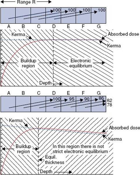
FIGURE 6.28. Schematic illustrating ionization measurement in air to determine dose in free space. (From Khan FM. The physics of radiation therapy, 2 nd ed. Baltimore: Williams & Wilkins; 1994.)

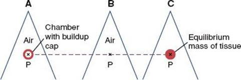
Determination of Absorbed Dose

It is difficult to measure absorbed dose directly, but two direct methods—calorimetry and Fricke dosimetry—are available in some laboratories. Neither method is particularly practical nor widely used, and the reader is referred to the literature for more details.⁶⁸ Instead, a simpler, indirect method using an exposure-calibrated ionization chamber is used to determine absorbed dose.

FIGURE 6.29. The roentgen-to-rad conversion factor for bone, muscle, and water as a function of photon energy. (From Johns HE, Cunningham JR. The physics of radiology, 4th ed. Springfield, IL: Charles C Thomas; 1983.)

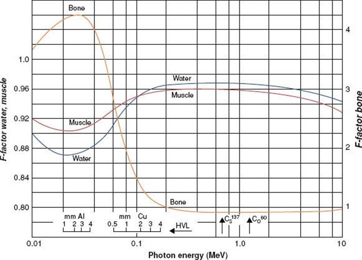
Absorbed Dose Calculation from Exposure Measurement

For photon energies of ⁶⁰Co and lower, an ionization chamber having an exposure calibration factor assigned by an appropriate national calibration facility (e.g., a dosimetry calibration laboratory accredited by the National Institute of Standards and Technology or the American Association of Physicists in Medicine [AAPM; College Park, MD]) can be used to measure exposure in air as described in the section Radiation Exposure. Absorbed dose then can be calculated from the exposure as explained here. The energy deposited in a fixed mass of air from a known exposure can be calculated because it is known that an exposure of 1 R creates a finite number of ion pairs per unit mass of air (i.e., 1.61 × 10¹⁵ ion pairs per kilogram of air) and that the mean energy required to create an ion pair in air (denoted by W) is equal to 33.97 eV per ion pair. When these values are used, the relationship between the exposure, X,and the dose to air, D_air, is given by the following expression:

The dose in free space, D_fs, is defined as the dose at the center of a small mass of phantom-like material just large enough to provide electronic equilibrium (Fig. 6.28) and can be derived from D_air using the ratio of the mass energy absorption coefficients (u_en/ρ) and an attenuation correction factor, A_eq, that accounts for the photon attenuation in the small mass of phantom-like material:

The term in brackets is called the f-factor or the roentgen-to-rad conversion factor and is represented as f_med, giving the dose in free space as follows:

Values of f_med are shown in Figure 6.29 over the energy range commonly used in radiation therapy. Notice that the f-factor is a function of the medium and the energy of the photon beam. Typical values of A_eqare 0.989 and 1.00 for ⁶⁰Co and 250-kV energies, respectively.

An in-air calibration procedure is performed as follows. The calibrated ion chamber (with wall thick enough to ensure electronic equilibrium) is placed in air with its sensitive volume on the central axis of the beam and its stem at right angles to the beam direction. The center of the chamber most often is placed at a distance from the source (or target) equal to the nominal SSD of the machine plus the buildup depth. A standard field size is set, usually 10 × 10 cm, using either movable collimators or the standard treatment applicator. An exposure is made for a known time or number of monitor units. The ionization chamber reading is converted to units of Gy/min at the depth of the maximum dose within a phantom, d_med, using the following equation:

where M, N_x, C_tp, C_st, C_s, A_eq, f_med, T, and α are used as defined earlier. The term TAR(d_max) represents the tissue–air ratio at the depth of maximum dose (i.e., the backscatter or peakscatter factor) and converts the dose in free space to the dose in a phantom at the depth of maximum dose. This parameter is discussed in more detail later. The preceding equation can be rewritten as follows:

and

This method is also valid when the measurements are made with the exposure-calibrated ion chamber embedded within a medium, such as a water phantom. In that case, the TAR(d_max) term is not included in the calculation, and the A_eq factor is replaced by a displacement factor, A_m. The numerical value of A_m is very close to that of A_eq, and for exposure measurements made within a water phantom, the dose rate is given by the following expression:

Absorbed Dose Calculation from Bragg–Gray Cavity Ionization Measurement

For energies above the level of ⁶⁰Co, exposure calibration factors are not available from the standards laboratories because of measurement limitations. In 1983, the AAPM introduced a protocol for the calibration of high-energy photon and electron beams that was based on Bragg–Gray cavity theory and allowed one to calculate dose directly from ion chamber measurements in a medium for energies above the level of ⁶⁰Co.⁶⁹ The protocol updated physical parameters and procedures for calibration and measurement and accounted for the different phantom materials (e.g., plastic and water) used for calibration and differences in ion chamber design and construction. The protocol introduced the cavity-gas calibration factor, N_gas, which is related to the ion chamber’s ⁶⁰Co exposure-calibration factor, N_x, and is used in conjunction with restricted stopping-power ratios, L^–/r, for the radiation beam in question to convert the ionization reading to absorbed dose using the following expression:

where M is the raw ionization chamber reading per monitor unit corrected for temperature and pressure, P_ion is the ion recombination correction factor, P_repl is a correction factor for replacement of phantom material by the ionization chamber, and P_wall is a correction factor to account for ionization chamber wall composition.

In 1999, the AAPM published a new protocol (TG-51) for the calibration of high-energy photon and electron beams.⁷⁰ This protocol uses ion chambers with absorbed-dose-to-water calibration factors, , which are traceable to national primary standards via the ⁶⁰Co standard. The absorbed dose to water at the point of measurement of the ion chamber placed under reference conditions is given by the following equation:

where Q is the beam quality of the clinical beam, M is the fully corrected ion chamber reading, and k_Q is the quality conversion factor that converts the calibration factor for a ⁶⁰Co beam to that for a beam of quality Q. The protocol is designed to be a simplification of the AAPM’s TG-21 protocol in the sense that large tables of stopping-power ratios and mass-energy absorption coefficients are no longer needed, and the user does not need to calculate any theoretical dosimetry factors.⁷¹^–⁷³

Other Dosimetry Methods

Thermoluminescence Dosimetry

Certain crystalline materials exhibit a phenomenon known as thermoluminescence. When a crystal capable of thermoluminescence is irradiated, a small portion of the energy absorbed is stored in the structure of the crystal lattice. If the material is heated, the energy is released in the form of visible light. Several thermoluminescent phosphors are available, but lithium fluoride, with an effective atomic number of 8.2, is the most commonly used.

The physical theory of thermoluminescence dosimetry can be explained as follows. In the individual atom, electrons occupy discrete energy levels. However, in the crystal lattice, the electronic energy levels are perturbed by mutual interactions between atoms, giving rise to energy bands, so-called allowed energy bands and forbidden energy bands. Impurities in the crystal create energy traps in the forbidden bands, allowing metastable states to exist; for example, when the phosphor is irradiated, some of the electrons in the valence band (ground state) receive sufficient energy to be raised to the conduction band. If there is an instantaneous emission of light, the phenomenon is called fluorescence. If an electron in the trap requires energy to get out of the trap and return to the valence band, the emission of light is called phosphorescence. If the emission of light is slow at room temperature but can be sped up with heating, the process is called thermoluminescence.

Thermoluminescence dosimeters must be calibrated before they can be used for measuring an unknown dose. Because the response of the thermoluminescent material is affected by its radiation and thermal histories, the material must be annealed to remove residual effects. The standard preirradiation annealing procedure for lithium fluoride is 1 hour of heating at 400°C and 24 hours at 80°C. More details can be found in the review article by DeWerd et al.⁷⁴

Film Dosimetry

When an x-ray film is exposed to ionizing radiation, the exposed silver bromide crystals form a latent image. In the film development process, the affected crystals cause a darkening of the film, and the unaffected crystals leave the film clear. The degree of blackening of the film is proportional to the energy absorbed and is measured by determining the optical density with a densitometer. The optical density is defined as follows:

where I₀ is the amount of light detected without the film in place and I_T is the amount of light detected with the film in place. For radiation dosimetry, the net optical density is obtained by subtracting the densitometric reading for the base fog (clear portion of the film) from the measured optical density. Most films are exposed to yield an optical density between 1.3 and 1.7 for optimal viewing.

A plot of net optical density as a function of radiation exposure or dose is called the sensitometric curve or the Hunter–Driffield (H-D) curve. If the curve is nonlinear, appropriate corrections must be applied to convert net optical density to absorbed dose.

The use of film is a relatively straightforward method of dosimetry for electron beams, but it must be done with extreme care in photon dosimetry. The problem is that the photoelectric effect depends on Z³ (Z_silver = 47), and the film emulsion strongly absorbs radiation below 100 kV. A concise review of radiographic film dosimetry can be found in the article by Das.⁷⁵

Radiochromic Film Dosimetry

Radiochromic film consists of a thin (7 to 23 mm), radiosensitive, colorless leuco dye bonded to a 100-mm-thick Mylar base. Radiochromic films are colorless before irradiation and turn deep blue when irradiated without physical, chemical, or thermal processing. The film is approximately tissue equivalent, integrates simultaneously at all measurement points, and has a high spatial resolution (>1,200 lines/mm). It shows a stable, reproducible response if protected from ultraviolet light, unstable temperatures, and humidity. Because radiochromic dye is an aromatic hydrocarbon, like plastic scintillators, it has an energy response superior to that of diodes and comparable with thermoluminescence dosimetry. Interest in radiochromic film as a quantitative dosimeter has been stimulated by the appearance of a fourfold-more-sensitive film (model MD-55), which extends its response down to the 5-Gy level. More details on radiochromic film dosimetry are given in the article by Soares et al.⁷⁶

Diode Dosimetry

Semiconductor diodes offer many advantages for clinical dosimetry, including high sensitivity, real-time read-out, robustness, and independence of air pressure. Most semiconductor diodes are made from silicon, which is either ntype (silicon doped with group V material, such as phosphorus) or p type (silicon doped with group III material, such as boron). To form a diode detector, a p-n junction must be created.

The physical theory of semiconductor dosimetry can be explained as follows. During irradiation, electron–hole pairs are created both within and outside the depletion region in the body of the diode detector. The charge carriers are swept across the depletion region and collected rapidly under the action of the electric field that exists across it. In this way, a current is generated, flowing in the reverse direction to normal diode current flow, which can be measured and related to absorbed dose.

Dosimetry diodes are operated without an external reverse bias voltage and connected via cable to a simple electrometer. Details on their use for in vivo dosimetry are provided in AAPM Report 87.⁷⁷ Calibration of diodes typically is performed by comparison of readings against an ion chamber in a standard setup to establish a diode calibration factor for absorbed dose to water and the establishment of a series of correction factors to account for calibration differences when measurements are performed under various experimental conditions. Typical concerns are energy dependence, temperature sensitivity, directional dependence, and radiation damage. Each radiation therapy center should establish the responses of their diodes under the various conditions encountered and monitor them as the cumulative dose to the diodes increases. Frequency of checks should be adjusted according to the frequency of use of the diodes and the variability encountered. More details on diode dosimetry are given in the article by Zhu and Saini.⁷⁸

Metal Oxide Semiconductor-Field Effect Transistor Dosimetry

Metal oxide semiconductor-field effect transistors represent another example of a semiconductor dosimeter. Originally developed for space dosimetry, the operation is based on the buildup of charge in the silicon oxide transistor gate created by ionizing radiation. The reader is referred to the article by Cygler and Scalchi⁷⁹ for more details on this type of dosimeter.

Polymer-Gel Dosimetry

Gel dosimetry is based on quantifying the effects of radiation-induced chemical changes occurring within some volume of material filled with an aqueous gel matrix. The degree of chemical change in the gel is related to dose. The dose-dependent changes are determined by imaging techniques, including magnetic resonance imaging, CT, and optical CT. Hence, gel dosimetry has the potential to provide full 3D dosimetry throughout the volume of the irradiated gel dosimeter.

For example, one form of this method exploits the radiation-induced free-radical chain polymerization of acrylic monomers dispersed in an aqueous gel. When irradiated, discrete, microscopic regions of cross-linked polymer are formed, the concentration of which is proportional to radiation dose. The water proton nuclear magnetic resonance relaxation rates in the gel are strongly affected by local changes in the polymer molecular structure and dynamics; thus, the distribution of radiation dose may be visualized and quantified with high resolution using MRI. Because the polymer microparticles scatter light, the dose distribution also can also be visualized in the transparent gel as a dose-dependent 3D optical turbidity and read by optical CT.

Unfortunately, gel dosimetry, while having the potential for tissue-equivalent 3D dosimetry for a little over two decades, has not come into common clinical use, as it as proven too difficult to use in the clinic setting.⁸⁰ Research continues in gel dosimetry, as there is clearly a need for a robust 3D high-resolution dosimetry system.⁸⁰^,⁸¹

FIGURE 6.30. Schematic drawing illustrating definition of percentage depth dose, where d is any depth and d₀ is the reference depth, usually d_max.

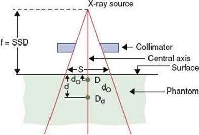
DOSIMETRY PARAMETERS

Percentage Depth Dose

Percentage depth dose (PDD) can be understood by reference to Figure 6.30. It is the ratio, expressed as a percentage, of the absorbed dose on the central axis at depth d to the absorbed dose at the reference point d₀. Percentage depth dose is given by

The functional symbols have been inserted in the expression to make it clear that the PDD is affected by a number of parameters, including d, d₀, field dimension S, source-to-surface distance f, and radiation beam energy (or quality) E. S refers to the side length of a square beam at a specified reference depth. Nonsquare beams may be designated by their equivalent square. Field shape and added beam collimation also can affect the central axis depth–dose distribution. Photon-beam PDD increases with increasing energy, SSD, and field size. Figure 6.31 shows that the depth of the 50th percentile increases from approximately 14 cm for 4-MV x-rays to nearly 23 cm for 25-MV x-rays. The depth of maximum dose varies from about 1 cm for 4-MV x-rays to >3.5 cm for 25-MV x-rays.

The PDD for one SSD is related to the PDD at a second SSD by the following equation:

The term in the brackets is called the Mayneord F-factor.⁸²

Tissue–Air Ratio

The tissue–air ratio (TAR) is defined as the ratio of the absorbed dose D_d at a given point in the phantom by the absorbed dose in free space, D_fs, that would be measured at the same point but in the absence of the phantom, if all other conditions of the irradiation (e.g., collimator, distance from the source) are equal (Fig. 6.32). The TAR is expressed as follows:

where d is depth, E is radiation beam energy, and S_d is the beam dimension measured at depth d. TAR depends on depth, field size, and beam quality, but for all practical purposes it is independent of the distance from the source.

The TAR at the depth of maximum dose is called the peakscatter factor. It is perhaps better known as the backscatter factor, but because of the finite depth d₀, this tends to be misleading. Figure 6.33 shows the peakscatter factors for various field sizes and beam qualities.

FIGURE 6.31. Examples of central axis percentage depth dose (DD) for megavoltage x-ray beams ranging from ⁶⁰Co to 18-MV x-rays and 6- to 20-MeV electron beams.

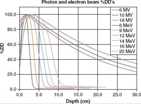
FIGURE 6.32. Schematic drawing illustrating the definition of tissue–air ratio, where d is the thickness of overlying material.

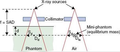
FIGURE 6.33. Variation of peakscatter factor with beam quality (half-value layer). (From Johns HE, Cunningham JR. The physics of radiology, 4th ed. Springfield, IL: Charles C Thomas; 1983.)

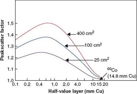
Tissue–Phantom Ratio and Tissue–Maximum Ratio

The concepts of tissue–phantom ratio (TPR) and tissue–maximum ratio (TMR) were proposed for high-energy radiation as alternatives to TAR in response to arguments raised against the use of in-air measurement for a photon beam with a maximum energy >3 MeV.⁸³^,⁸⁴ As originally defined, TPR is given by the ratio of two doses:

where is the dose at a specified point on the central axis in a phantom with a fixed reference depth, d_r, of tissue-equivalent material overlying the point; D_d is the dose in the phantom at the same spatial point as before but with an arbitrary depth, d, of overlying material; and S_d is the beam width at the level of measurement (Fig. 6.34). In each instance, underlying material is sufficient to provide for full backscatter. There is no general agreement about the magnitude of the reference depth to be used for this quantity, particularly for high energies. The TPR is intended to be analogous to the TAR but has an advantage because the reference dose, , is directly measurable over the entire range of x-rays and γ-rays in use, eliminating problems in obtaining a value for the dose in free space when the depth for electronic buildup is great.

The original TMR definition is similar to the definition of TPR, except that the reference depth, d_r, is the depth of maximum dose. However, the depth of maximum dose for megavoltage x-ray beams varies significantly with field size and also is a function of SSD. Thus, the definition of TMR creates a measurement problem because a variable d_r is required and the TMR depends on SSD. A modification by Khan et al.⁸⁵ proposed that the reference depth, d_r, must be equal to or greater than the largest depth of maximum dose.

Purdy⁸⁶ reported on the relationships between the central axis percentage depth dose and the TPR, TMR, and TAR. This work suggested that the degree to which the TPR and TMR are independent of distance from the radiation source depends largely on the linac’s collimator/flattening-filter scatter component of the beam.

Scatter–Air Ratio and Scatter–Maximum Ratio

The scatter-air ratio (SAR) can be thought of as the scatter component of the TAR.⁸⁷ It is defined as follows:

SAR is the difference between the TAR for a field of finite area and the TAR for a zero-area field size. The zero-area TAR is a mathematical abstraction obtained by extrapolation of the TAR values measured for finite field sizes.

Similarly, the scatter-maximum ratio (SMR), the scatter component of the TMR, is defined as follows:

where S_p is a phantom scatter correction factor, which takes into account changes in scatter radiation originating in the phantom at the reference depth as the field size is changed.⁸⁵

FIGURE 6.34. Schematic drawing illustrating the definition of tissue–phantom ratio and tissue–maximum ratio, where d is the thickness of overlying material and d_r is the reference thickness.

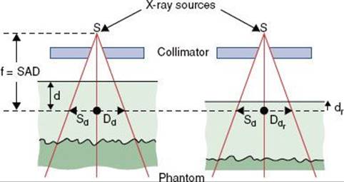
Output Factor

The output factor for a given field size is defined as the ratio of the dose rate at the depth of maximum dose for a given field size to that for the reference field size (usually 10 × 10 cm) at its d_max. The output factor varies with field size (Fig. 6.35) as a result of two distinct phenomena. As the collimator jaws are opened, the primary dose, D_p, at d_max on the central ray per monitor unit increases as a result of a larger number of primary x-ray photons scattered out of the flattening filter. In addition, the scatter dose, D_s(d_max, r), at the measurement point per unit D_p increases as the scattering volume irradiated by primary photons increases with increasing collimated field size. These two components can vary independently of one another if nonstandard treatment distances or extensive secondary blocking is used.

Khan et al.⁸⁵ described a method for separating the overall output factor, S_c,p, into two components. One is the collimator scatter factor, S_c(r_c), which is a function only of the collimator opening, r_c, projected to isocenter. The other is the phantom scatter factor, S_p(r), which is a function only of the cross-sectional area or effective field size, r, irradiated at the treatment distance. They demonstrate that

In practice, the total and collimator scatter factors both are measured and the phantom scatter factor is calculated using the relationship listed previously. S_c(r_c) is measured in air using an ion chamber fitted with an equilibrium-thickness buildup cap and given by the ratio of the reading for the given collimator opening to the reading for a reference field (typically 10 × 10 cm) collimator opening. The overall output factor is measured in-phantom using the standard treatment distance and is given by the reading relative to that for a 10 × 10 cm field size. By carefully extrapolating this measured ratio to zero-field size, one obtains the zero-field-size phantom scatter factor, S_p(0). If a small-ion chamber is positioned axially in the beam, it is possible to measure S_c,p for field sizes as small as 1 × 1 cm. Because of the loss of lateral secondary electron equilibrium encountered near the edges of high-energy photon beams, S_p deviates significantly from unity. Consistent separation of primary and scatter dose components significantly improves the accuracy of dose predictions for irregular field calculations, especially near block edges and the resultant dose falloff resulting from lateral electron disequilibrium, and under blocks, overcoming many of the dose-modeling problems presented by use of extensive customized blocking.

Isodose Curves

An isodose curve represents points of equal dose. A set of these curves, normally given in 10% increments normalized to the dose at the reference depth, can be plotted on a chart (i.e., isodose chart) to give a visual representation of the dose distribution in a single plane (Fig. 6.36). Beam parameters, such as source size, flattening filter, field size, and SSD, play important roles in the shape of the isodose curve.

Dose Profiles

A dose profile is a representation of the dose in an irradiated volume as a function of spatial position along a single line. Dose profiles are particularly well suited to the description of field flatness and penumbra. The data most often are given as ratios of doses normalized to the dose on the central axis (Fig. 6.37). The profiles, called off-axis factors or off-center ratios, may be measured in air (i.e., with only a buildup cap) or in a phantom at selected depths. The in-air off-axis factor gives only the variation in primary beam intensity; the in-phantom off-center ratio shows the added effect of phantom scatter.

FIGURE 6.35. Example of output factor as a function of lower and upper collimator settings for a medical linear accelerator 18-MV x-ray beam.

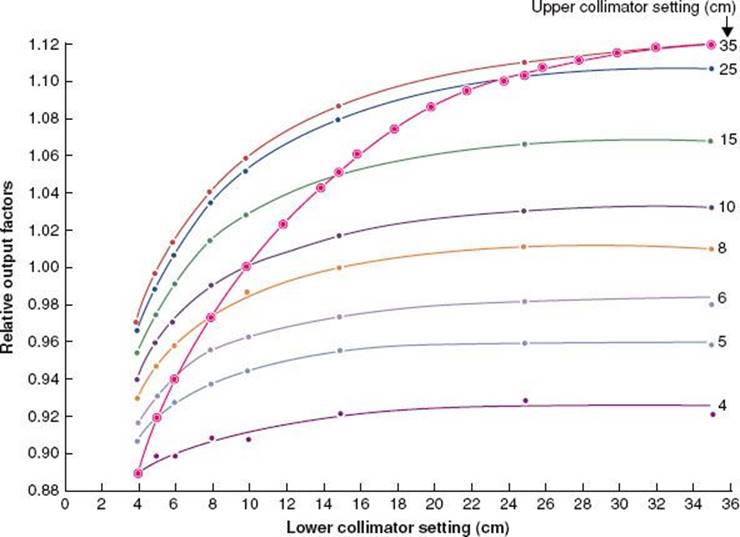
FIGURE 6.36. Isodose distributions for different quality radiations. A: 200 kVp, source–skin distance (SSD) = 50 cm, half-value layer (HVL) = 1 mm Cu, field size = 10 × 10 cm. B: ⁶⁰Co, SSD = 80 cm, field size = 10 × 10 cm. C: 4-MV x-rays, SSD = 100 cm, field size = 10 × 10 cm. D: 10-MV x-rays, SSD = 100 cm, field size = 10 × 10 cm. (From Khan FM. The physics of radiation therapy, 3rd ed. Baltimore: Williams & Wilkins; 1994.)

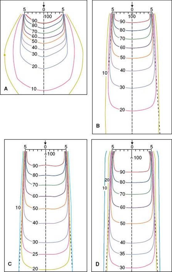
Wedge Filter

Wedge filters, first introduced by Ellis and Miller,⁸⁸ generally are constructed of brass, steel, or lead. When placed in the beam they progressively decrease intensity across the field, causing the isodose distribution to have a planned asymmetry.

The wedge angle is defined as the angle the isodose curve subtends with a line perpendicular to the central axis at a specific depth and for a specified field size. Current practice is to use a depth of 10 cm. Past definitions were based on the 50th-percentile isodose curve and, more recently, the 80th-percentile isodose curve. The wedge angle is a function of field size and depth. The wedge factor is defined as the ratio of the dose measured in a tissue-equivalent phantom at the depth of maximum buildup on the central axis with the wedge in place to the dose at the same point with the wedge removed.

Wedge isodose curves can be normalized in different ways, as shown in Figure 6.38. The wedged isodose distribution on the left side of the figure has been normalized to 100% at d_max on the central axis with the wedge in place; on the right, the normalization is done without the wedge in place. Thus, it is imperative that the normalization and the use of the wedge factor should be clearly understood before wedges are used clinically.

Beam hardening occurs when a wedge is inserted into the radiation beam. The PDD, therefore, can be considerably increased at depth. Differences in PDD of nearly 7% have been reported for a 4-MV x-ray, 60-deg wedge field, compared with the open field at a depth of 12 cm, and there have been reports of as much as a 3% difference between the 60-deg wedge field and the open field for a 25-MV x-ray beam.⁸⁹^,⁹⁰

FIGURE 6.37. Example of dose profiles for an 18-MV linear accelerator x-ray beam measured at depths of 3 and 10 cm.

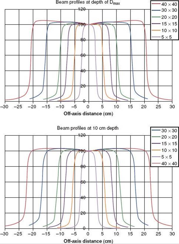
FIGURE 6.38. Isodose curves for a wedge filter. A: Normalized to D_max. B: Normalized to D_max without the wedge. ⁶⁰Co, wedge angle = 45 deg, field size = 8 × 10 cm, source–skin distance = 80 cm. (From Khan FM. The physics of radiation therapy, 3rd ed. Baltimore: Williams & Wilkins; 1994.)

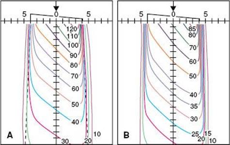
REFERENCES

1. Khan FM. The physics of radiation therapy. 4th ed. Philadelphia: Lippincott Williams & Wilkins; 2010.

2. Podgorsak EB. Radiation physics for medical physicists, 2nd ed. Berlin: Springer; 2010.

3. Van Dyk J, ed. The modern technology of radiation oncology. Madison, WI: Medical Physics Publishing; 1999.

4. Williams JR, Thwaites DI. Radiotherapy physics: in practice, 2nd ed. Oxford: Oxford University Press; 2000.

5. Van Dyk J, ed. The modern technology of radiation oncology, Vol. 2. Madison, WI: Medical Physics Publishing; 2005.

6. Roentgen WC. A new kind of rays [in German]. Sitzungber Phys Med Ges (Wurzburg) 1895;137.

7. Becquerel H. Emission de radiations nouvilles par l’uranium métallique. C R Acad Sci Paris 1896;122:1086.

8. Curie P, Curie M, Belmont MG. Sur une nouvelle substance fortement radio-active, contenue dans la pechblende. C R Hebdomadaires Séances Acad Sci Paris 1898;127:1215.

9. Paganetti H, Niemierko A, Ancukiewicz M, et al. Relative biological effectiveness (RBE) values for proton beam therapy. Int J Radiat Oncol Biol Phys 2002;53(2):407–421.

10. Biggs P, Ma C-M, Doppke K, et al. Kilovoltage x-rays. In: Van Dyk J, ed. The modern technology of radiation oncology. Madison, WI: Medical Physics Publishing; 1999:287–312.

11. Aumock A, Birnbaum EH, Fleshman JW, et al. Treatment of rectal adenocarcinoma with endocavitary and external beam radiotherapy: results for 199 patients with localized tumors. Int J Radiat Oncol Biol Phys2001;51(2):363–370.

12. Purdy JA, Prasad SC, Walz BJ, et al. Radiation protection considerations for endocavitary. Int J Radiat Oncol Biol Phys 1985;11:2177–2181.

13. Schulz MD. The supervoltage story. Am J. Roentgenol Radium Ther Nucl Med 1975;124:541–559.

14. Kerst DW. The betatron. Radiology 1943;40:120–127.

15. Karzmark CJ, Nunan CS, Tanabe E. Medical electron accelerators. New York: McGraw-Hill; 1993.

16. Johns HE, Bates IM, Watson TA. 1000 curie cobalt units for radiation therapy. I. The Saskatchewan cobalt-60 unit. Br J Radiol 1952;25:296.

17. Green DT, Errington RF. Design of a cobalt 60 beam therapy unit. Br J Radiol 1952;25:309.

18. Glasgow GP. Cobalt-60 teletherapy. In: Van Dyk J, ed. The modern technology of radiation oncology. Madison, WI: Medical Physics Publishing; 1999:313–348.

19. Leksell L. Cerebral radiosurgery: I. Gammathalamotomy in two cases of intractable pain Acta Chir Scand 1968;134:585–595.

20. Miller CW. Traveling-wave linear accelerator for x-ray therapy. Nature 1953;171:297–298.

21. Howard-Flanders P. The development of the linear accelerator as a clinical instrument. Acta Radiol 1954;116:649–655.

22. Ginzton EL, Mallory KB, Kaplan HS. The Stanford medical linear accelerator. I. Design and development. Stanford Med Bull 1957;15:123–140.

23. Podgorsak EB, Metcalfe P, Van Dyk J. Medical accelerators. In: Van Dyk J, ed. The modern technology of radiation oncology. Madison, WI: Medical Physics Publishing; 1999:349–435.

24. Klein EE, Taylor M, Michaletz-Lorenz M, et al. A mono-isocentric technique for breast and regional nodal therapy using dual asymmetric jaws. Int J Radiat Oncol Biol Phys 1994;28:753–760.

25. Leavitt DD, Martin M, Moeller JH, et al. Dynamic wedge field techniques through computer-controlled collimator motion and dose delivery. Med Phys 1990;17:87–91.

26. American Association of Physicists in Medicine. Report 72: Basic applications of multileaf collimators: Report of Task Group 50 of the Radiation Therapy Committee. Madison, WI: Medical Physics Publishing; 2001.

27. Klein EE, Harms WB, Low DA, et al. Clinical implementation of a commercial multileaf collimator: dosimetry, networking, simulation, and quality assurance. Int J Radiat Oncol Biol Phys 1995;33:1195–1208.

28. Intensity Modulated Radiation Therapy Collaborative Working Group. NCI IMRT Collaborative Working Group: Intensity modulated radiation therapy: current status and issues of interest. Int J Radiat Oncol Biol Phys2001;51(4):880–914.

29. Jaffray DA, Drake DG, Moreau M, et al. A radiographic and tomographic imaging system integrated into a medical linear accelerator for localization of bone and soft-tissue targets. Int J Radiat Oncol Biol Phys 1999;45:773–789.

30. Jaffray DA, Siewerdsen JH, Wong JW, et al. Flat-panel cone-beam computed tomography for image-guided radiation therapy. Int J Radiat Oncol Biol Phys 2002;53(5):1337–1349.

31. Rao M, Yang W, Chen F, et al. Comparison of Elekta VMAT with helical tomotherapy and fixed field IMRT: plan quality, delivery efficiency and accuracy. Med Phys 2010;37(3):1350–1359.

32. Ling CC, Zhang P, Archambault Y, et al. Commissioning and quality assurance of RapidArc radiotherapy delivery system. Int J Radiat Oncol Biol Phys 2008;72(2):575–581.

33. Yu CX. Intensity modulated arc therapy with dynamic multileaf collimation: an alternative to tomotherapy. Phys Med Biol 1995;40(9):1435–1449.

34. Yu CX, Tang G. Intensity-modulated arc therapy: principles, technologies and clinical implementation. Phys Med Biol 2011;56(5):R31–R54.

35. Ling CC, Archambault Y, Bocanek J, et al. Scylla and Charybdis: longer beam-on time or lesser conformality—the dilemma of tomotherapy. Int J Radiat Oncol Biol Phys 2009;75(1):8–9.

36. Mehta M, Hoban P, Mackie TR. Commissioning and quality assurance of RapidArc radiotherapy delivery system: in regard to Ling et al. (Int J Radiat Oncol Biol Phys 2008;72;575–581): absence of data does not constitute proof; the proof is in tasting the pudding. Int J Radiat Oncol Biol Phys 2009;75(1):4–6.

37. Veksler VJ. A new method for acceleration of relativistic particles [in Russian]. Dokl Akad Nauk SSSR 1944;43:329.

38. Schwinger J. On the classical radiation of accelerated electrons. Phys Rev 1949;75:1912–1925.

39. Brahme A. Design principles and clinical possibilities with a new generation of radiation therapy equipment. Acta Oncol 1987;26:403–412.

40. Mackie TR, Holmes T, Swerdloff S, et al. Tomotherapy: a new concept for the delivery of dynamic conformal radiotherapy. Med Phys 1993;20(6):1709–1719.

41. Jeraj R, Mackie TR, Balog J, et al. Radiation characteristics of helical tomotherapy. Med Phys 2004;31(2):396–404.

42. Adler JR, Chang SD, Murphy MJ, et al. The CyberKnife: a frameless robotic system for radiosurgery. Stereotactic Functional Neurosurg1997;69:124–128.

43. Adler JR, Murphy MJ, Chang SD, et al. Image-guided robotic radiosurgery. Neurosurgery 1999;44:1299–1307.

44. Kamino Y, Takayama K, Kokubo M, et al. Development of a four-dimensional image-guided radiotherapy system with a gimbaled x-ray head. Int J Radiat Oncol Biol Phys 2006;66(1):271–278.

45. Depuydt T, Verellen D, Haas O, et al. Geometric accuracy of a novel gimbals based radiation therapy tumor tracking system. Radiother Oncol 2011;98(3):365–372.

46. Kirkby C, Stanescu T, Rathee S, et al. Patient dosimetry for hybrid MRI-radiotherapy systems. Med Phys 2008;35(3):1019–1027.

47. DesRosiers C, Moskvin V, Bielajew AF, et al. 150–250 MeV electron beams in radiation therapy. Phys Med Biol 2000;45:1781–1805.

48. Fuchs T, Szymanowski H, Oelfke U, et al. Treatment planning for laser-accelerated very-high energy electrons. Phys Med Biol 2009;54:3315–3328.

49. Wilson RW. Radiological use of fast protons. Radiology 1946;47:487–491.

50. Breuer H, Smit BJ. Proton therapy and radiosurgery. Berlin: Springer-Verlag; 2000.

51. Delaney TF, Kooy HM. Proton and charged particle radiotherapy. Philadelphia: Lippincott Williams & Wilkins; 2008.

52. Schulz-Ertner D, Jakel O, Schlegel W. Radiation therapy with charged particles. Sem Radiat Oncol 2006;16(4):249–259.

53. Coutrakon G, Bauman M, Lesyna D, et al. A prototype beam delivery system for the proton medical accelerator at Loma Linda. Med Phys 1991;18((6)):1093–1099.

54. Hall EJ. Intensity-modulated radiation therapy, protons, and the risk of second cancer. Int J Radiat Oncol Biol Phys 2006;65(1):1–7.

55. Henning W, Shank C, eds. Accelerators for America’s future. Washington, DC: U.S. Department of Energy; 2010.

56. Caporaso GJ, Mackie TR, Sampayan S, et al. A compact linac for intensity modulated proton therapy based on a dielectric wall accelerator. Phys Med 2008;24(2):98–101.

57. Maughan RL, Powers WE. A superconducting cyclotron for neutron radiation therapy. Med Phys 1994;21(6):779–785.

58. Maughan RL, Yudelev M. Neutron therapy. In: Van Dyk J, ed. The modern technology of radiation oncology. Madison, WI: Medical Physics Publishing; 1999:871–917.

59. Van Dyk J, Munro PN. Simulators. In: Van Dyk J, ed. The modern technology of radiation oncology. Madison, WI: Medical Physics Publishing; 1999:95–129.

60. Nishidai T, Nagata Y, Takahashi M, et al. CT simulator: A new 3-D planning and simulation system for radiotherapy. I. Description of system. Int J Radiat Oncol Biol Phys 1990;18:499–504.

61. Perez CA, Purdy JA, Harms WB, et al. Design of a fully integrated three-dimensional computed tomography simulator and preliminary clinical evaluation. Int J Radiat Oncol Biol Phys 1994;30(4):887–897.

62. Sherouse GW, Bourland JD, Reynolds K, et al. Virtual simulation in the clinical setting: some practical considerations. Int J Radiat Oncol Biol Phys 1990;19(4):1059–1065.

63. Van Dyk J, Taylor JS. CT simulators. In: Van Dyk J, ed. The modern technology of radiation oncology. Madison, WI: Medical Physics Publishing; 1999:131–168.

64. Mutic S, Palta JR, Butker EK, et al. Quality assurance for computed-tomography simulators and the computed-tomography-simulation process: Report of the AAPM Radiation Therapy Committee Task Group No. 66. Med Phys2003;30(10):2762–2792.

65. Mutic S, Purdy JA, Michalski JM, et al. The simulation process in the determination and definition of the treatment volume and treatment planning. In: Levitt SH, Purdy JA, Perez CA, et al., eds. Technical basis of radiation therapy. Berlin: Springer; 2006:107–133.

66. Almond P. A historical perspective: a brief history of dosimetry, calibration protocols, and the need for accuracy. In: Rogers DWO, Cygler JE, eds. Clinical dosimetry measurements in radiotherapy.Madison, WI: Medical Physics Publishing; 2009:1×27.

67. Orton CG, Seibert JB. The measurement of teletherapy unit timer errors. Phys Med Biol 1972;17:198.

68. Kron T. Dose measuring tools. In: Van Dyk J, ed. The modern technology of radiation oncology. Madison, WI: Medical Physics Publishing; 1999:753–821.

69. American Association of Physicists in Medicine, Task Group 21, Radiation Therapy Committee. A protocol for the determination of absorbed dose from high-energy photon and electron beams. Med Phys1983;10:741–771.

70. Almond PR, Biggs PJ, Coursey BM, et al. AAPM’s TG-51 protocol for clinical reference dosimetry of high-energy photon and electron beams. Med Phys 1999;26:1847–1870.

71. Huq MS, Andreo P. Reference dosimetry in clinical high-energy photon beams: comparison of the AAPM TG-51 and AAPM TG-21 dosimetry protocols. Med Phys 2001;28(1):46–54.

72. Huq MS, Andreo P, Song H. Comparison of the IAEA TRS-398 and AAPM TG-51 absorbed dose to water protocols in the dosimetry of high-energy photon and electron beams. Phys Med Biol2001;46(11):2985–3006.

73. Huq MS, Song H. Reference dosimetry in clinical high-energy electron beams: comparison of the AAPM TG-51 and AAPM TG-21 dosimetry protocols. Med Phys 2001;28(10):2077–2087.

74. DeWerd LA, Bartol LJ, Davis SD. Thermoluminescent dosimetry. In: Rogers DWO, Cygler JE, eds. Clinical dosimetry measurements in radiotherapy. Madison, WI: Medical Physics Publishing; 2009:815–840.

75. Das IJ. Radiographic Film. In: Rogers DWO, Cygler JE, eds. Clinical dosimetry measurements in radiotherapy. Madison, WI: Medical Physics Publishing; 2009:865–890.

76. Soares CG, Trichter S, Devic S. Radiochromic film. In: Rogers DWO, Cygler JE, eds. Clinical dosimetry measurements in radiotherapy. Madison, WI: Medical Physics Publishing; 2009:759–813.

77. American Association of Physicists in Medicine. Report 87. Diode in Vivo Dosimetry for Patients Receiving External Beam Radiation Therapy: Report of Task Group 62 of the Radiation Therapy Committee. Madison, WI: Medical Physics Publishing; 2005.

78. Zhu TC, Saini AS. Diode dosimetry for megavoltage electron and photon beams. In: Rogers DWO, Cygler JE, eds. Clinical dosimetry measurements in radiotherapy. Madison, WI: Medical Physics Publishing; 2009:913–939.

79. Cygler JE, Scalchi P. MOSFET dosimetry in radiotherapy. In: Rogers DWO, Cygler JE, eds. Clinical dosimetry measurements in radiotherapy. Madison, WI: Medical Physics Publishing; 2009:941–977.

80. Baldock C, De Deene Y, Doran S, et al. Polymer gel dosimetry. Phys Med Biol 2010(55):R1–R51.

81. Schreiner LJ, Olding T. Gel dosimetry. In: Rogers DWO, Cygler JE, eds. Clinical dosimetry measurements in radiotherapy. Madison, WI: Medical Physics Publishing; 2009:979–1025.

82. Burns JE. Conversion of depth doses from one FSD to another. Br J Radiol 1958;31:643.

83. Holt JD, Laughlin JS, Moroney JP. The extension of the concept of tissue-air (TAR) to high energy x-ray beams. Radiology 1970;96:437–446.

84. Karzmark CJ, Deubert A, Loevinger R. Tissue-phantom ratios—an aid to treatment planning. Br J Radiol 1965;38:158-159.

85. Khan FM, Sewchand W, Lee J, et al. Revision of tissue-maximum ratio and scatter-maximum ratio concepts for cobalt 60 and higher energy x-ray beams. Med Phys 1980;7:230–237.

86. Purdy JA. Relationship between tissue-phantom ratio and percentage depth dose. Med Phys 1977;4:66.

87. Cunningham JR. Scatter-air ratios. Phys Med Biol 1972;17:42–51.

88. Ellis F, Miller H. The use of wedge filters in deep x-ray therapy. Br J Radiol 1944;17:90.

89. Abrath FG, Purdy JA. Wedge design and dosimetry for 25-MV x rays. Radiology 1980;136:757–762.

90. Sewchand W, Khan FM, Williamson J. Variations in depth-dose data between open and wedge fields for 4-MV x rays. Radiology 1978;127:789–792.

Page

Contents

If you find an error or have any questions, please email us at admin@doctorlib.org. Thank you!