Lesya M. Shuba,
Young H. Kwon
Glaucoma is a condition characterized by optic neuropathy and a corresponding visual field loss. This loss is usually very insidious and starts in the periphery leaving patients asymptomatic in the early stages. Having a sensitive and specific test to detect a subtle visual field loss is therefore very important in glaucoma management. Visual field evaluation is a complex task that has become an integral part of the glaucoma evaluation. There are two main reasons to conduct a visual field examination in patients with suspected or established glaucoma: (1) to make the diagnosis and (2) to determine visual field stability in follow-up. Recently, several new promising visual field testing modalities have become available. Early diagnosis and detection of disease progression still remain challenging.
HILL OF VISION
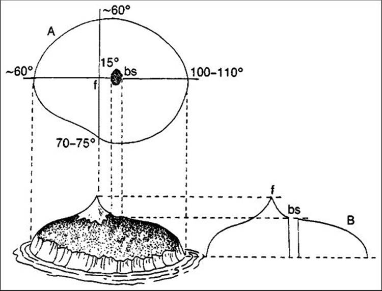
In 1939, Traquair[1] cleverly described a normal visual field as 'an island of vision surrounded by a sea of blindness' (Fig. 196.1). The 'top of the island' corresponds to the fovea with the highest light sensitivity (fixation point); it declines toward the periphery, and the bottom corresponds to the peripheral visual field with the lowest light sensitivity. The normal visual field has an oval shape: temporal field extends to 100-110°, inferior to 70-75°, and superior and nasal to 60° (Fig. 196.1). An area of visual loss within the visual field is called scotoma. If the loss of vision is total, the scotoma is absolute; if it is partial, the scotoma is relative. A blind spot is an absolute scotoma corresponding to the optic nerve head and is located ?15° temporal to the fovea (Fig. 196.1).
|
|
|
|
FIGURE 196.1 Normal visual field described by Traquair as 'an island of vision surrounded by a sea of blindness'. The 'top of the island' corresponds to the center of fixation - fovea (f). The blind spot (bs) corresponds to the optic nerve head and is located 15° temporal to the fovea. The dimensions of the normal visual field are shown in (A). |
TYPES OF PERIMETRY
Standard visual field testing involves measuring the contrast sensitivity, or the ability of an observer to just distinguish the target from the background. The light intensity or luminance is measured in apostilbs (asb); 1 asb corresponds to 0.318 candela/square meter (cd/m2). Decibels are logarithmic relative units which indicate the degree of attenuation of the maximal light intensity that the instrument can produce. The absolute intensity of a light expressed in dB (equal to 0.1 log unit) is determined by the maximum possible illumination of a specific light source. Thus, if a maximum possible light intensity of a source is 10000 asb, a 30 dB (or 3 log unit attenuation) light corresponds to 10 abs, a 10 dB (or 1 log unit attenuation) to 1000 abs, and 0 dB (or no attenuation) to 10000 abs. This also means that threshold detection of a 30 dB stimulus (very dim light) indicates a higher retinal sensitivity than 10 dB (brighter light).
Conventional visual field testing is performed with a white target against a more dimly illuminated white background ('white-on-white' or Standard Achromatic Perimetry (SAP)). In the two commonly used perimeters (Humphrey and Goldmann), the background illumination is kept steady at 31.5 asb and stimulus size and intensity are altered. Two main types of SAP currently used in clinical practice are kinetic and static.
MANUAL KINETIC PERIMETRY
Manual kinetic perimetry is usually done using a Goldmann perimeter[2] which consists of a bowl with a radius of 30 cm. Both stimulus size and intensity can be adjusted (Table 196.1). The subject is asked to fixate on a central target in the bowl while a trained technician monitors fixation. The technician steadily (4° per second) brings a stimulus of a certain size and intensity from a non-seeing area until the subject indicates that the stimulus is seen. The process is repeated for stimuli of different size and intensity creating a number of isopters. An isopter represents a circular line on a visual field within which a light target of a certain size and intensity is visible.
TABLE 196.1 -- Stimulus Sizes in Goldmann Perimetry
|
Goldmann Stimulus Size |
Area on 30 cm Bowl (mm2) |
Angle Subtended (°) |
|
0 |
1/16 |
0.05 |
|
I |
1/4 |
0.11 |
|
II |
1 |
0.22 |
|
III |
4 |
0.43 |
|
IV |
16 |
0.86 |
|
V |
64 |
1.72 |
The Armaly-Drance technique was developed specifically for glaucoma screening, and it tests areas of the visual field which have the highest probability of being damaged in the disease.[2-6] The technique uses a suprathreshold static perimetry in the central 25° and kinetic stimuli in the periphery with the emphasis on the nasal-horizontal meridian. This technique has been shown to be highly sensitive and specific.[4,5]
The careful examination of a visual field using a Goldmann perimeter is time consuming and requires a highly trained technician. However, it allows for a careful peripheral examination, and some patients, especially the elderly or those with advanced field loss, perform better on manual perimeters compared to automated devices. Summary Box 1 lists relative advantages of the manual and automated perimetry.
Summary Box 1
|
Advantages of manual kinetic perimetry:
Advantages of automated static perimetry
|
AUTOMATED STATIC PERIMETRY
GENERAL OVERVIEW
In the last half of the twentieth century, several automated perimeters became available. Currently, the most widely used one is a Humphrey Field Analyzer (HFA), and the most common type is static perimetry.[7] In static perimetry, stimuli of the same size and different intensity are randomly presented in predetermined locations of the visual field and subject responses are registered. Of note, HFA is capable of performing automated kinetic perimetry, but it is not commonly used. Computerized automated static perimetry has several advantages including reduced operator variability, shorter test duration, and the ability to perform sophisticated statistical analysis of the results (Summary Box 1).
Automated perimetry using HFA can be performed using any one of the five stimulus sizes (I-V) corresponding to the Goldmann perimeter (Table 196.1). The default stimulus is size III. For a patient who has advanced glaucomatous loss documented with a size III stimulus, it is reasonable to switch to size V to increase the dynamic range of the test (Key Feature 1).
Key Feature 1
|
In patients with advanced glaucomatous loss consider
|
Currently, most practitioners examine the central 24°. Compared to a 30° field, examining 24° eliminates only one row of peripheral points (except for the 2 nasal most points), but shortens the test duration by 10-20%, which is always a desirable outcome in perimetry (Table 196.2). In central 24° and 30° fields, test stimuli are presented in a 6° grid. In 24-1 and 30-1 patterns, test stimuli are presented along the horizontal and vertical meridians and then every 6°.[8] In more commonly used 24-2 and 30-2 patterns, the test stimuli are presented 3° away from the horizontal and vertical meridians and then every 6°.[8]HFA also offers an option of examining only the central 10° with a 2° test grid. This can offer useful information in patients with advanced disease, who have only a small intact central island, and in those with a small central defect. To further increase a dynamic range of a 10° field, the stimulus size can be increased from III to V (Key Feature 1).
TABLE 196.2 -- Testing Algorithms in Humphrey Field Analyzer
|
30-2 |
24-2 |
10-2 |
|
|
Number of test points |
76 |
54 |
68 |
|
Grid |
6° |
6° |
2° |
|
SITA |
Available |
Available |
Available |
THRESHOLD TESTING
Full Threshold Strategy
In automated perimetry, threshold values are defied as stimuli intensity detected 50% of the time. In the Full Threshold strategy, stimuli are presented at predetermined locations using a 4-2 algorithm where the threshold is crossed twice - initially in 4 dB increments followed by 2 dB increments. Examination of the central 24° visual field using this technique takes 15-20 min. In the rapid threshold program, FASTPAC, the threshold is crossed only once and in 3 dB steps. While this decreases the test duration by ?35%, it also reduces the accuracy.
Swedish Interactive Threshold Algorithms
The goal of any test of the visual function is to improve test sensitivity and specificity. In the world of perimetry, one way to achieve this is by improving test reliability and variability by decreasing test duration without sacrificing the quality of the results. Recently, this has been accomplished using a Swedish Interactive Threshold Algorithm (SITA). This testing strategy is available on the HFA II (Humphrey Systems, Dublin, CA). The SITA strategy uses more efficient mathematical methods for estimation of threshold values based on normative data, patient age, and patient responses during the test. The threshold values are adjusted in real time during the test, and pace is altered depending on the patient response speed.[9-11] The test time is also reduced by eliminating retest trials for short-term fluctuation determination and redundant questioning for assessing false positive (FP) and false negative (FP) responses. By using this 'smart' strategy of dynamic testing adjustment, SITA-Standard reduced the test duration by ?50% compared to the Full Threshold strategy. Importantly, this reduction in the test duration is not done by sacrificing quality; SITA matches and even surpasses the accuracy of the Full Threshold strategy.[10-16]To further decrease the test duration by 30-50%, SITA-Fast strategy was designed. However, test-retest reliability for this strategy is worse compared to SITA-Standard.[12-14] Currently, the most common clinically used strategy of SAP is the SITA-Standard.
RELIABILITY
Patient's cooperation and understanding of a test are critical for test reliability.[7] So, it is wise before the first visual field test to spend extra time with patients explaining the purpose and the basic technique of the perimetry. To decrease anxiety, patients need to understand that it is normal not to see about half of the stimuli presented, but at the same time, they need to respond even when the stimulus is just barely perceptible.
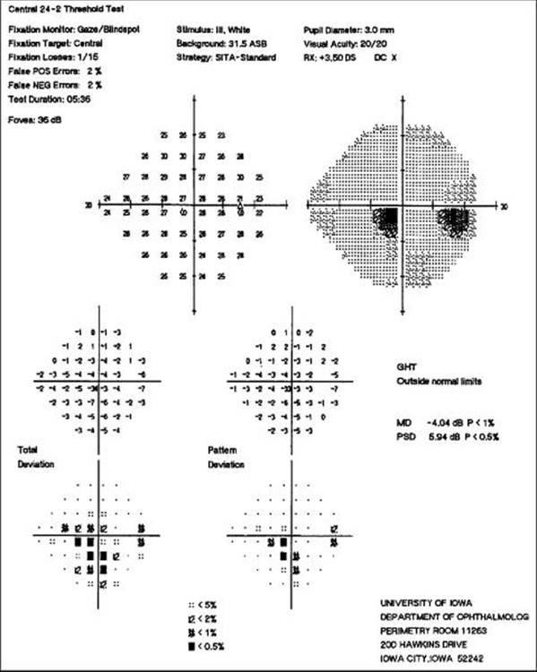
Interpretation of any visual field should start with the analysis of reliability indices (Summary Box 2). These indices are located in the upper-left corner of the Single Field Analysis printout (Fig. 196.2). It is also important to note any remarks that a perimetrist may have written on a printout. Below are the reliability indices available on a Full Threshold and SITA printouts. Note that these two strategies use different methods to assess test reliability (Tip File 1).
Summary Box 2
|
Test reliability measures:
|
|
|
|
|
FIGURE 196.2 The Single Field Analysis printout of a central 24-2 SITA-Standard obtained with the HFA on a patient with an inferior paracentral scotoma. The top part of the printout provides general information about the test and the patient (strategy, stimulus size, patient's date of birth etc). The reliability indices are shown in the left upper corner. Grayscale and numeric threshold plots (in dB) are shown under the general test information. TD and PD numeric (dB) and probability plots are presented in the left lower corner. To the right of the plots are GHT (GHT which is outside normal limits in this patient) and Global Indices (MD and PSD). |
Tip File 1
|
Full Threshold and SITA strategies use different methods for monitoring fixation and test reliability. |
Fixation Losses
Maintaining central fixation is very important for mapping an accurate and reproducible visual field. Several methods of fixation monitoring are available on the HFA II (Summary Box 2). A technician can monitor a patient's eye on a screen to ensure a steady fixation. When a 'Fixation Monitor' is set at 'blind spot', a Heijl-Krakau technique[17] is used, where stimuli are projected several times during a test into an area of a previously mapped blind spot. If a patient responds to such stimuli, it is assumed to be a fixation loss. Fixation losses exceeding 20% of the total trials are flagged. When interpreting these results, it is important to ensure that the blind spot was mapped correctly at the beginning of the test (Tip File 2). Another source of error in this method is patient head tilt during the test. Even a small tilt can move the blind spot and result in artificially high fixation losses. HFA II also has an option of a gaze tracker where the alignment of corneal reflexes and pupil is used to assess subject's fixation throughout the test.
Tip File 2
|
When interpreting fixation losses determined using the Heijl-Krakau technique, ensure that the blind spot was mapped correctly at the beginning of the test. |
FP Errors
In a Full Threshold or FASTPAC strategy, False positive (FP) errors are registered when a patient responds to a catch trial in which an auditory stimulus is given in the absence of a visual stimulus. FP errors are recorded as a percentage of responses from catch trials and are flagged if they are higher than 33%. Patients with high FP errors may be overly anxious and reassuring them that it is normal to miss ?50% of the stimuli can usually cure 'trigger happy' patients. SITA does not use 'catch trials' to register FP, instead, it calculates them as responses that occurred outside the normal response time window.
FN Errors
In a Full Threshold or FASTPAC strategy, False negative (FN) errors are recorded when a patient does not respond to stimuli 9 dB brighter than previously registered at that location. FN errors are recorded as a percentage of responses and are flagged if they are higher than 33%. Two most common causes of increased FN are: (1) patient fatigue (can produce a 'cloverleaf field') and (2) end-stage glaucoma (Key Feature 2). High levels of FN errors in advanced glaucoma are thought to be secondary to significant short-term and long-term fluctuation (Figs 196.3 and 196.4) associated with the disease.[7] SITA does not spend extra time during a test on catch trial; instead, FN errors are estimated at the end of the test as stimuli when, during threshold testing, a patient denied seeing a stimulus that was later found to be brighter. Only test points from the relativelynormal parts of the visual field are considered in this analysis. Therefore, unlike FN errors obtained in the Full Threshold strategy, those estimated in SITA should not be elevated in end-stage glaucoma, but only in inconsistent subjects.[7]
Key Feature 2
|
Two most common causes of increased FN:
Unlike FN errors obtained in the Full Threshold strategy, those estimated in SITA should not be elevated in end-stage glaucoma but only in inconsistent subjects. |
|
|
|
|
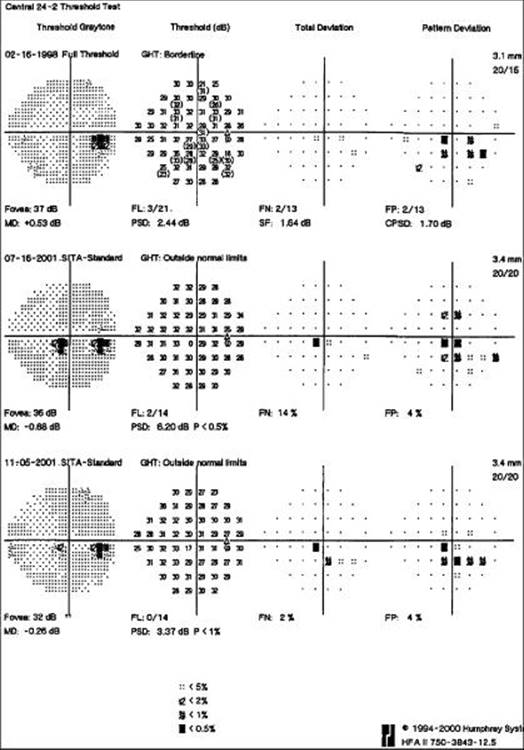
FIGURE 196.3 The overview printout of the same patient as in Figure 196.2 presents three visual fields done over a period of almost 4 years (16 Feb 1998 to 5 Nov 2001). The first field shows a suggestion of an inferior paracentral scotoma; this scotoma becomes more prominent on the second field and less prominent on the third one, just to become more prominent again in 2006 (Fig. 196.2). Such long-term fluctuation is typical in patients with glaucoma. |
|
|
|
|
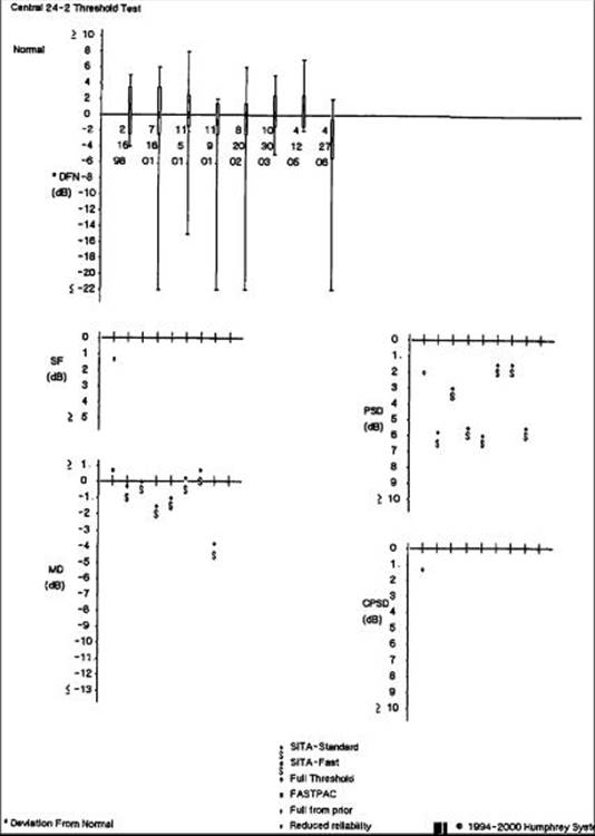
FIGURE 196.4 The Change Probability Analysis of the same patient as in Figures 196.2 and 196.3. The box plot is presented at the top. This patient has a small, deep scotoma; therefore the boxes are normal size, but have long negative tails. In some fields (30 Oct 2003 and 12 Apr 2005) the negative tails disappear, again demonstrating long-term fluctuation in this patient. The long-term fluctuation is also evident on the chronological plots of MD and PSD (bottom). |
VISUAL FIELD PLOTS
Threshold sensitivity values (dB) are plotted from stimuli presentations at predetermined test locations.
The grayscale is a schematic representation of threshold values. It helps to appreciate a general pattern of the visual field and draws attention to abnormal areas which require further careful studying. It is important to realize that the most commonly used spot size in automated Humphrey 24-2 or 30-2 visual field is 0.43° (size III), and the stimuli are presented in a 6° grid. Therefore, the shading between the test points on the grayscale represents interpolated threshold values. The grayscale plot should be examined with caution since it is easily influenced by many artifacts (Key Feature 3).[7]
Key Feature 3
|
The grayscale plot should be examined with caution since it is easily influenced by many artifacts. |
Total Deviation (TD) plots are calculated as a difference between the patient's threshold values and those of the age-matched normals. Points on a visual field close to fixation have a narrow range of normal values, while those on the periphery have a wider range. Therefore, TD plots are center-weighted such that an abnormal central point is assigned more significance than a peripheral point. These are presented as a dB plot (top left plot on The Single Field Analysis) and as a probability plot (bottom left plot on The Single Field Analysis) (Fig. 196.2).
Pattern Deviation (PD) dB and probability plots are located to the right of the TD plots on The Single Field Analysis printout (Fig. 196.2). PD is calculated by adjusting the overall sensitivity (TD values) of the visual field by the seventh-most sensitive non-edge point, to differentiate focal defects from generalized changes. Therefore, PD plots highlight focal visual field defects and ignore generalized changes (Key Feature 4).[7]
Key Feature 4
|
PD plots highlight focal visual field defects and ignore generalized changes. |
GLOBAL INDICES (SUMMARY BOX 3)
Mean Deviation (MD) represents an average deviation of the patient's visual field from the age-matched controls. Its calculation is center-weighted. A negative MD indicates a depressed field, while a positive value represents a higher than normal sensitivity. MD does not help in differentiating diffuse from focal loss.
Summary Box 3
|
Global indices:
|
Pattern Standard Deviation (PSD) represents the degree of irregularity in the field. The higher the value the more uneven is the field indicating a focal visual field defect. Usually an increase in PSD in a patient with glaucoma suggests progression. However, in end-stage disease, MD may continue to decrease (i.e., become more negative), but PSD may start to decrease or 'improve' (Key Feature 5). This may initially give a physician a false sense of stability, but it indicates a severe disease when the irregularity in the visual field is slowly lost because the whole field is becoming evenly depressed ('floor effect').
Key Feature 5
|
In progressing end-stage glaucoma, MD may continue to decrease, but PSD may also start to decrease ('improve'). |
Short Term Fluctuation (STF) is available in the Full Threshold, but not in the SITA strategy. It represents the consistency of patient responses during a single test and is determined by retesting the same ten points.
Corrected Pattern Standard Deviation (CPSD) represents a PSD corrected for STF. This is done in the attempt to eliminate irregularities in the visual field secondary to unreliable patient responses. It is available in the Full Threshold but not in the SITA strategy.
ARTIFACTS
There are several variables, other than disease, that may influence a visual field (Summary Box 4). The first visual field for a patient is usually not very reliable and often shows visual field defects that are not confirmed on later testing. The learning curve for visual field testing is steep for most patients.
Summary Box 4
|
Visual field artifacts:
|
Diffuse visual field loss can be secondary to media opacities or a small pupil. The most common media opacity affecting the visual field in glaucoma patients is cataract. Progression of a cataract tends to cause a generalized depression of the visual field (i.e., worsening TD and MD) without any localized loss (i.e., stable PD and PSD). Similar generalized depression is observed in patients with small pupils. If the pupil size is less than 3 mm, it should be dilated pharmacologically before the test.
Several visual field artifacts can be caused by different refractive errors. Central visual field testing requires a near add, the power of which depends on patient age and is calculated by HFA II. A diffuse visual field loss may be secondary to an uncorrected refractive error. It is important to follow HFA manual instructions on the use of trial lenses including proper centration and positioning. Improper alignment of trial lenses can cause a lens rim artifact resulting in a peripheral ring scotoma.
Upper lid ptosis can cause a superior visual field loss. In contrast to a superior arcuate scotoma, such a defect does not connect with the blind spot and disappears after upper lid retraction or taping.
Since the TD plot is calculated based on age-matched normative data, incorrect entry of patient age can result in very abnormal TD, PD, MD, and PSD. Therefore, a review of any visual field should start at the top of The Single Field Analysis printout which includes patient's date of birth.
An overly anxious 'trigger happy' patient, in addition to having high FP errors, will often have unrealistically high threshold levels producing 'white scotomas'. Be aware when interpreting PD plots in such patients. A cursory look at such visual fields may erroneously give the impression of a localized visual field defect registered on PD plot. This, however, is only due to an artificially elevated hill of vision produced by unrealistically high thresholds.
DETECTION AND MONITORING PROGRESSION
Detecting progression in a chronic and slowly progressive disease is challenging. Monitoring visual fields is only one means of assessing progression. In following visual fields in glaucoma patients, it is often difficult to differentiate between normal short-term and long-term fluctuation (Figs 196.3 and 196.4) and true disease progression. Because of such high variability, a new change on a visual field needs to be confirmed on repeat testing.[7,18,19]
HFA II comes equipped with a statistical software, STATPACT, which is capable of analyzing a single visual field for abnormalities or a series of fields for progression (Summary Box 5).
Summary Box 5
|
Analysis of visual fields:
|
The Single Field Analysis provides a printout of a single visual field with the most detailed information about that test (Fig. 196.2).
In the Overview printout, several visual fields are arranged chronologically on the same page for the ease of comparison (Fig. 196.3).
The Change Analysis printout provides a chronologic box plot analysis, the time courses of the four global indices (only MD and PSD in SITA), and the linear regression analysis of MD.[7] (Fig. 196.4)
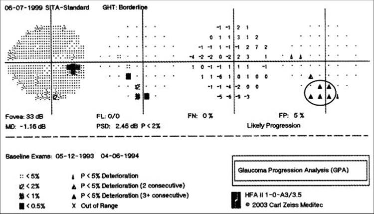
The Glaucoma Progression Analysis (GPA) uses the point analysis of the sequential visual fields to differentiate early, true progression from long-term fluctuation (Fig. 196.5). The normal long-term fluctuation used for the analysis was determined from a large group of stable glaucoma patients and was found to depend on the overall MD, and depth and location of the defect.[7,20] The program compares patient's follow-up visual fields with the selected baseline exams. Obviously, it is important to select truly representative fields as a baseline; otherwise all future comparisons will not be useful. The follow-up visual fields are subtracted from the baseline to create a deviation from baseline plot (change in pattern deviation, dB) (Fig. 196.5, third column) and a GPA plot (Fig. 196.5, fourth column). On the GPA plot, open triangles indicate points that have worsened at the p<5% significance level; half-filled and filled triangles indicate points that have worsened at the p<5% significance level in two or three follow-up exams, respectively. When significant deterioration occurs in the same three or more points on two consecutive fields, the GPA AlertT interprets it as a 'Possible Progression'. If such deterioration occurs in three consecutive fields, it is interpreted as a 'Likely Progression' (Fig. 196.5).
|
|
|
|
FIGURE 196.5 The GPA identifies an early change in the visual field, typical of glaucoma. The five points (circled) showed significant deterioration in three consecutive tests (filled triangles) resulting in a GPA AlertT of Likely Progression. |
The Glaucoma Hemifield Test (GHT) is used to identify localized visual field defects typical of glaucoma.[7,21-22] In the test, both inferior and superior hemifields are divided into five zones, and the average threshold values of the superior and inferior mirror images are compared. Five different outcomes of the GHT are possible: (1) GHT within normal limits; (2) GHT borderline; (3) GHT outside normal limits; (4) General reduction of sensitivity; and (5) Abnormally high sensitivity (Key Feature 6).
Key Feature 6
|
The GHT outcomes:
|
OTHER PERIMETRIC TECHNIQUES
SAP remains the mainstay of glaucoma diagnosis and follow-up; however, as evident from the previous discussion, it has its limitations. It has been recognized that almost 40% of retinal ganglion cells may die before a visual field defect is detected on a SAP.[23,24] The search for new, more sensitive, and specific tests to assess function in glaucoma continues.[25-32] The ideal new modalities should be able not only to specifically detect glaucoma at early stages, but also be effective at monitoring progression. Recently, several new, promising techniques have been developed.[25-28,31,33-35]
To improve the sensitivity of visual field testing, the new modalities are aimed at stimulating only a discrete type of ganglion cells. The classification of ganglion cells is incomplete and complex. There are at least three types of retinal ganglion cells: midget, parasol, and small bistratified ganglion cells (Table 196.3).[29,36,37] All three types of cells are stimulated during SAP. This causes significant redundancy and probably, loss of sensitivity. The newer techniques of visual field assessment attempt to stimulate only a specific type of retinal ganglion cells.[25,29,37] Some of these methods are discussed below.
TABLE 196.3 -- Retinal Ganglion Cell Types
|
Midget Ganglion Cells |
Parasol Ganglion Cells |
Bistratified Ganglion Cells |
|
|
Distribution |
70% |
8-10% |
6-10% |
|
Size |
Small |
Large |
Small |
|
LGN projections |
Parvocellular layers |
Magnocellular layers |
Interlaminar zones of the parvocellular layer |
|
Other names |
P cells |
M cells |
|
|
Function |
High resolution tasks, color, low-temporal and high spatial frequencies |
Motion, and high temporal and low spatial frequencies |
Short wavelength blue stimuli |
SHORT WAVELENGTH AUTOMATED PERIMETRY
It is believed that patients with glaucoma develop a tritan-like (blue-green) deficiency.[38-40] This observation led to the development of Short Wavelength Automated Perimetry (SWAP). SWAP is available on the HFA II (Humphrey Systems, Dublin, CA, USA). SWAP is designed to isolate the short wavelength (blue) pathway. It uses large, blue stimuli which are presented on the bright yellow background. A number of studies have demonstrated that SWAP is able to detect glaucomatous damage earlier than SAP.[25,27,41-47]
Some studies noted that SWAP produces greater variability, including higher short- and long-term fluctuation, compared to SAP.[48-51] The dynamic range of the SWAP perimetry is narrower than that of SAP. While SWAP is good at detecting early glaucomatous damage and progression, it is not very suitable for follow up of patients with moderate or advanced disease.[30] The results obtained with SWAP are influenced by the absorption of the short wavelength light by the cataractous lens. Hence, it may be difficult with SWAP to differentiate a glaucomatous diffuse visual field loss from that due to cataract.
Full threshold SWAP testing used to be very long and tiring for patients. SITA algorithm recently became available for SWAP on the HFA II, decreasing test duration to 3-6 min.[52] In addition, SITA SWAP appears to have higher sensitivities, increasing the dynamic range of the test, and reducing the inter-subject variability.[53]
FREQUENCY DOUBLING PERIMETRY
There is evidence suggesting that large M-type ganglion cells are preferentially affected in early glaucoma.[54] Frequency Doubling Perimetry (FDT) was developed with the hope of early glaucoma detection based on the theory of initial loss of M-type ganglion cells. First FDT machines (FDT1) tested the central visual field with only 17 or 19 test points using a large stimulus size (10°).[33] Recently, Humphrey Matrix became available (FDT2; Humphrey Systems, Dublin CA, USA). FDT2 uses the same number of stimuli (54 in a 24° field) as SAP. The stimuli are 5° squares of black and white grading with a low spatial frequency which undergo a counter-phase flicker at a high temporal frequency. This results in a 'frequency doubling' phenomenon which, some believe, isolates a subset of M ganglion cells - My cells.[29]
FDT has been shown to be resistant to refractive blur[33,55] but not to the effects of cataract.[56] The test appears to be highly specific and sensitive in detecting early, moderate, and advanced glaucomatous visual field damage.[57-60] Several studies showed that FDT is able to detect glaucomatous damage before the SAP,[25,36,41,61] while others feel that FDT and SAP detect dif-ferent visual field defects.[62]Overall, FDT may be a good adjunct for diagnosis and follow up of patients with glaucoma.[55] There is also evidence that it may be suitable for glaucoma screening.[63,64]
Landers and colleagues[41] compared SWAP, FDT, and SAP in detecting visual field deficits in ocular hypertensive patients. They found that the results of SWAP and FDT highly correlated, and that both tests found defects before they were registered with SAP. Similarly, Sample and colleagues[36] found that in a group of eyes with glaucomatous optic neuropathy, SWAP and FDT identified higher percentage of visual fields as abnormal, compared to SAP.
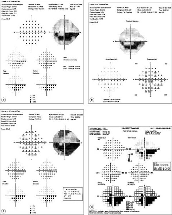
Figure 196.6 shows visual fields of a patient with an inferior arcuate scotoma obtained using SAP (stimulus size III and V), SWAP, and FDT. Table 196.4 compared SAP, SWAP, and FDT on a number of different features.
|
|
|
|
FIGURE 196.6 Examples of visual fields of a patient with an inferior arcuate scotoma obtained on the same day using different techniques: SAP stimulus size III (a), SAP stimulus size V (b), SWAP (c), and FDT Matrix (d). The scotoma was smaller and less dense on the SAP stimulus size V compare to stimulus size III visual field. The diffuse loss was more pronounced with SWAP compared to SAP and FDT, but the focal loss (i.e., PD) was similar between the techniques. |
TABLE 196.4 -- Different Techniques of Automated Perimetry
|
SAP SITA |
SWAP SITA |
FDT2 |
|
|
Test duration |
4-6 min with SITA |
4-6 min with SITA |
4-6 min |
|
Early detection |
Poor |
Good |
Good |
|
Patient preference |
Moderate |
Poor, but improved with SITA |
Better than SAP |
|
Sensitivity |
Moderate |
High |
High |
|
Effect of cataract |
Yes |
Yes |
Yes |
|
Experience |
Old |
New |
New |
|
Ganglion cell types |
All |
Bistratified |
M type |
|
Variability |
Moderate |
High |
Moderate |
|
Stimulus size |
Usually 0.43° (4 mm2, Goldmann III) |
1.8° (64 mm2, Goldmann V) |
5° square |
|
Stimulus type |
Broadband visible light, maximum intensity 10 000 Asb; duration 200 ms |
Blue light (440 nM), maximum intensity 65 Asb; duration 200 ms |
Black and white grading with a spatial frequency of 0.5 cyc/deg counterphase at 18 Hz; duration 500 ms |
|
Background |
White 10 cd/m2 (31.5 Asb) |
Yellow 100 cd/m2 (315 Asb) |
White 100 cd/m2 (315 Asb) |
|
Early vs moderate vs advanced glaucoma |
Good for moderate/advanced |
Good for early |
Good for early/moderate/advanced |
GLAUCOMATOUS VISUAL FIELD LOSS
RETINAL ORGANIZATION OF THE NERVE FIBER LAYER
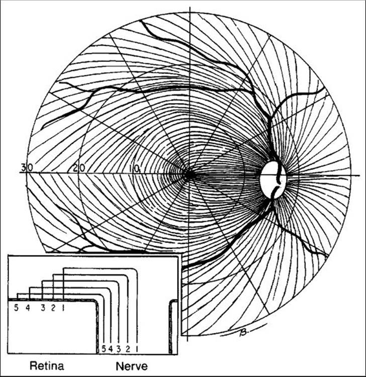
Understanding the pattern of visual loss in glaucoma requires the knowledge of the retinal nerve fiber layer organization in relation to the optic nerve morphology. The nerve fibers are organized in such way that the temporal visual field is represented by the nasal retina, nasal visual field by the temporal retina, and so on. The nerve fiber layer also has a characteristic topographic layout (Fig. 196.7). Because of the particular topographic organization of the nerve fiber layer, glaucomatous optic neuropathy leads to typical visual field defects in the distribution of retinal nerve fiber bundles (Key Feature 7).
|
|
|
|
FIGURE 196.7 Characteristic topographic organization of the retinal nerve fiber layer of the right eye. The ganglion cell axons from the macula area form a papillomacular bundle which enters directly at the temporal side of the optic disk. The axons from the temporal retina have to arch around the papillomacular bundle and enter the optic nerve at the inferior and superior poles. The axons from the nasal retina enter the optic nerve radially on the nasal side. |
Key Feature 7
|
The typical glaucomatous visual field defect occurs in the distribution of a retinal nerve fiber bundle. |
CHARACTERISTIC VISUAL FIELD LOSS
Before the early 1980s, most of the visual field studies were performed manually, using either the tangent screen or the Goldmann perimeter.[65] Manual perimetric examinations for early, localized visual field loss found that the early paracentral scotoma was the most characteristic type of shallow or, perhaps, fleeting visual field loss in early glaucoma.[66,67] In an investigation of 53 patients who experienced visual field loss while under study, Werner and Drance[68] found that localized defects often were preceded by inconsistent responses in the region that subsequently would acquire the scotoma (Tip file 3). Hart and Becker[69] found that 53% of the initial defects in 800 patients with glaucoma were in the superior or inferior arcuate region, extending from the blind spot to the horizontal raphe in an arc that was between 5° and 15° from fixation. The degree of visual field loss is usually different between the superior and inferior hemifields.[7] This asymmetry is the basis of the GHT (discussed earlier).
Tip File 3
|
One of the earliest presentations of glaucomatous visual field loss can be increase in short-term (intra-test) and long-term (inter-test) fluctuations. |
LOCALIZED VISUAL FIELD LOSS (SUMMARY BOX 6)
Paracentral scotomas (within central 10°) are a common early presentation of glaucoma (especially in normal tension glaucoma, see Figs 196.2 and 196.3). Because they follow a nerve fiber layer distribution, they terminate at the horizontal raphe.
Summary Box 6
|
Glaucomatous localized visual defects:
|
A nasal (Roenne) step represents an area of reduced sensitivity in the nasal field which respects the horizontal raphe (Fig. 196.8a).
|
|
|
|
FIGURE 196.8 Examples of glaucomatous visual field defects obtained with HFA: (a) Inferior nasal (Roenne) step. (b) Superior hemifield loss. (c) Advanced-stage glaucoma. |
Arcuate (Bjerrum) scotoma can develop as an extension of a paracentral scotoma toward the blind spot (Fig. 196.6). Enlargement of arcuate scotoma can lead to a hemifield loss (Fig. 196.8b).
Regardless of the initial site at which visual field loss is detected, the defects tend to enlarge and deepen and follow the nerve fiber bundle pattern as they progress. A ring scotoma is formed when the inferior and superior arcuate defects join. In advanced-stage glaucoma, only central and temporal islands of vision may remain (Fig. 196.8c). Overall, the decline in visual field in treated glaucoma patients is slow: ?1.3 to ?2% (Goldmann) or ?0.11 to ?0.35 dB (Humphrey) per year.[70-73]
When a patient presents with one of the typical visual field defects described above, the diagnosis is easier. It is more challenging to recognize the earliest glaucomatous visual field changes before the typical pattern develops. Several methods for recognizing early visual field defects have been proposed, some of them are rather complicated for use in every day clinical practice but have been used in studies.[74] Anderson and Patella[7] suggested three criteria for minimal abnormality (Summary Box 7): (1) three or more non-edge points at the expected location with sensitivities at p < 5% and one point with sensitivity at p < 1%; or (2) PSD (or CPSD) at p < 5%; or (3) GHT indicating an abnormal field. Of course, these visual field changes must be reproducible and in keeping with other clinical fidings.
Summary Box 7
|
Criteria for minimal abnormality:
|
NORMAL TENSION VERSUS HIGH TENSION GLAUCOMA
It is thought that patients with normal tension glaucoma tend to have more localized visual field defects, whereas those with high tension glaucoma suffer more diffuse losses.[75-78]
However, Caprioli and associates[78] suggested that high intra-ocular pressure (IOP) alone is enough to prompt careful visual field evaluation and thus facilitate the fiding of diffuse visual field loss. Patients with low or normal IOP generally are less likely to be subjected to visual field examination, unless their optic nerve shows suspicious defects. Localized visual field loss correlates with localized disk notching or with vertical elongation of the optic cup, both of which are easier to detect by routine ophthalmoscopy than the more saucerized cups associated with diffuse visual field loss.[79] A patient with a pressure of 18 mmHg with a localized optic disk notch is more likely to undergo visual field examination, and a localized defect may be found. However, if a patient with a pressure of 18 mmHg has a saucerized optic cup, it may not trigger a visual field examination. Consequently, an associated diffuse visual field loss may be missed. Thus, there is a selection bias in favor of patients with low-tension glaucoma who have localized visual field defects. Careful study is needed to resolve this issue.
SUMMARY
Visual field testing remains an important tool in the diagnosis and follow-up of glaucoma. Visual fields used for the initial diagnosis of glaucoma must be sufficiently sensitive to detect abnormality early and must be sufficiently specific to ensure that an abnormal test is likely to predict the presence of the disease. Both manual and automated perimetric methods are capable of detecting glaucoma reliably. The former tend to be tedious and require a well-trained technician or physician to administer them. Even under optimal circumstances, examiner variability can have a negative impact on test reliability and reproducibility. For these reasons and others, computerized automated perimetry has become increasingly popular since 1980. In addition to its ability to decrease examiner variability by eliminating the examiner during the actual testing procedure, computerized perimeters can process data statistically and help the examiner interpret the results more reliably and quantitatively. The disadvantages are that computerized perimeters are expensive to purchase and maintain, and they are not as flexible as manual perimeters in performing patient-specific examinations. Recently, several new, promising visual field testing modalities have become available. Some of them offer earlier detection of glaucoma than SAP. However, at this time, SAP still remains the standard of care for glaucoma detection and follow-up.
Visual field testing is only one modality available in the management of glaucoma patients. When making decisions about diagnosis or treatment, other parameters such as IOP, optic disk analysis, patient age, and other risk factors should also be considered.
REFERENCES
1. Traquair HM: Clinical detection of early changes in the visual field. Trans Am Ophthalmol Soc 1939; 37:158-179.
2. Alward WL: In: Krachmer JH, ed. Glaucoma. The requisites in ophthalmology, Mosby; 2000.
3. Armaly MF: Ocular pressure and visual fields. A ten-year follow-up study. Arch Ophthalmol 1969; 81:25-40.
4. Rock WJ, Drance SM, Morgan RW: A modification of the Armaly visual field screening technique for glaucoma. Can J Ophthalmol 1971; 6:283-292.
5. Rock WJ, Drance SM, Morgan RW: Visual field screening in glaucoma. An evaluation of the Armaly technique for screening glaucomatous visual fields. Arch Ophthalmol 1973; 89:287-290.
6. Drance SM: The glaucomatous visual field. Br J Ophthalmol 1972; 56:186-200.
7. Anderson DR, Patella VM: Automated static perimetry, 2nd edn.. Mosby, 1999.
8. Humphrey Instruments I: In: Haley JH, ed. The field analyzer primer, 2nd edn.. Humphrey Instruments; 1987.
9. Bengtsson B, et al: A new generation of algorithms for computerized threshold perimetry, SITA. Acta Ophthalmol Scand 1997; 75:368-375.
10. Bengtsson B, Heijl A: Evaluation of a new perimetric threshold strategy, SITA, in patients with manifest and suspect glaucoma. Acta Ophthalmol Scand 1998; 76:268-272.
11. Bengtsson B, Heijl A, Olsson J: Evaluation of a new threshold visual field strategy, SITA, in normal subjects. Swedish Interactive Thresholding Algorithm. Acta Ophthalmol Scand 1998; 76:165-169.
12. Sekhar GC, et al: Sensitivity of Swedish interactive threshold algorithm compared with standard full threshold algorithm in Humphrey visual field testing. Ophthalmology 2000; 107:1303-1308.
13. Wild JM, et al: The SITA perimetric threshold algorithms in glaucoma. Invest Ophthalmol Vis Sci 1999; 40:1998-2009.
14. Artes PH, et al: Properties of perimetric threshold estimates from Full Threshold, SITA Standard, and SITA Fast strategies. Invest Ophthalmol Vis Sci 2002; 43:2654-2659.
15. Budenz DL, et al: Comparison of glaucomatous visual field defects using standard full threshold and Swedish interactive threshold algorithms. Arch Ophthalmol 2002; 120:1136-1141.
16. Budenz DL, et al: Sensitivity and specificity of the Swedish interactive threshold algorithm for glaucomatous visual field defects. Ophthalmology 2002; 109:1052-1058.
17. Heijl A, Krakau CE: An automatic static perimeter, design and pilot study. Acta Ophthalmol (Copenh) 1975; 53:293-310.
18. Anderson DR, Graham S, Pillunat L: Normal-tension glaucoma. J Glaucoma 2003; 12:164-166.
19. Schulzer M: Errors in the diagnosis of visual field progression in normal-tension glaucoma. Ophthalmology 1994; 101:1589-1594.discussion 1595.
20. Heijl A, Lindgren A, Lindgren G: Test-retest variability in glaucomatous visual fields. Am J Ophthalmol 1989; 108:130-135.
21. Katz J, et al: Automated perimetry detects visual field loss before manual Goldmann perimetry. Ophthalmology 1995; 102:21-26.
22. Asman P, Heijl A: Glaucoma hemifield test. Automated visual field evaluation. Arch Ophthalmol 1992; 110:812-819.
23. Quigley HA, Addicks EM, Green WR: Optic nerve damage in human glaucoma. III. Quantitative correlation of nerve fiber loss and visual field defect in glaucoma, ischemic neuropathy, papilledema, and toxic neuropathy. Arch Ophthalmol 1982; 100:135-146.
24. Quigley HA, Dunkelberger GR, Green WR: Retinal ganglion cell atrophy correlated with automated perimetry in human eyes with glaucoma. Am J Ophthalmol 1989; 107:453-464.
25. Sample PA, Johnson CA: Functional assessment of glaucoma. J Glaucoma 2001; 10(5 Suppl 1):S49-S52.
26. Johnson CA: Recent developments in automated perimetry in glaucoma diagnosis and management. Curr Opin Ophthalmol 2002; 13:77-84.
27. Sample PA: Short-wavelength automated perimetry: it's role in the clinic and for understanding ganglion cell function. Prog Retin Eye Res 2000; 19:369-383.
28. Johnson CA: Psychophysical measurement of glaucomatous damage. Surv Ophthalmol 2001; 45(Suppl 3):S313-S318.discussion S322-S324.
29. Shabana N, et al: Motion perception in glaucoma patients: a review. Surv Ophthalmol 2003; 48:92-106.
30. Wild JM, et al: Short wavelength automated perimetry the long-term fluctuation of the visual field in stable glaucoma. Acta Ophthalmol Scand 2001; 79:546-559.
31. Chauhan BC: Detection of glaucoma: the role of new functional and structural tests. Curr Opin Ophthalmol 2004; 15:93-95.
32. Anderson RS: The psychophysics of glaucoma: improving the structure/function relationship. Prog Retin Eye Res 2006; 25:79-97.
33. Anderson AJ, Johnson CA: Frequency-doubling technology perimetry. Ophthalmol Clin North Am 2003; 16:213-225.
34. Chauhan BC: The value of high-pass resolution perimetry in glaucoma. Curr Opin Ophthalmol 2000; 11:85-89.
35. Mansberger SL, et al: Predictive value of frequency doubling technology perimetry for detecting glaucoma in a developing country. J Glaucoma 2005; 14:128-134.
36. Sample PA, et al: Visual function-specific perimetry for indirect comparison of different ganglion cell populations in glaucoma. Invest Ophthalmol Vis Sci 2000; 41:1783-1790.
37. Sample PA: What does functional testing tell us about optic nerve damage?. Surv Ophthalmol 2001; 45(Suppl 3):S319-S324.discussion S332-S334.
38. Sample PA, Boynton RM, Weinreb RN: Isolating the color vision loss in primary open-angle glaucoma. Am J Ophthalmol 1988; 106:686-691.
39. Heron G, Adams AJ, Husted R: Foveal and non-foveal measures of short wavelength sensitive pathways in glaucoma and ocular hypertension. Ophthalmic Physiol Opt 1987; 7:403-404.
40. Heron G, Adams AJ, Husted R: Central visual fields for short wavelength sensitive pathways in glaucoma and ocular hypertension. Invest Ophthalmol Vis Sci 1988; 29:64-72.
41. Landers J, Goldberg I, Graham S: A comparison of short wavelength automated perimetry with frequency doubling perimetry for the early detection of visual field loss in ocular hypertension. Clin Experiment Ophthalmol 2000; 28:248-252.
42. Demirel S, Johnson CA: Incidence and prevalence of short wavelength automated perimetry deficits in ocular hypertensive patients. Am J Ophthalmol 2001; 131:709-715.
43. Casson EJ, Johnson CA, Shapiro LR: Longitudinal comparison of temporal-modulation perimetry with white-on-white and blue-on-yellow perimetry in ocular hypertension and early glaucoma. J Opt Soc Am A Opt Image Sci Vis 1993; 10:1792-1806.
44. Johnson CA, et al: Progression of early glaucomatous visual field loss as detected by blue-on-yellow and standard white-on-white automated perimetry. Arch Ophthalmol 1993; 111:651-656.
45. Johnson CA, et al: Blue-on-yellow perimetry can predict the development of glaucomatous visual field loss. Arch Ophthalmol 1993; 111:645-650.
46. Racette L, Sample PA: Short-wavelength automated perimetry. Ophthalmol Clin North Am 2003; 16:227-236.vi-vii.
47. Sample PA, Weinreb RN: Progressive color visual field loss in glaucoma. Invest Ophthalmol Vis Sci 1992; 33:2068-2071.
48. Hutchings N, et al: Long-term fluctuation in short-wavelength automated perimetry in glaucoma suspects and glaucoma patients. Invest Ophthalmol Vis Sci 2001; 42:2332-2337.
49. Wild JM, et al: Statistical aspects of the normal visual field in short-wavelength automated perimetry. Invest Ophthalmol Vis Sci 1998; 39:54-63.
50. Kwon YH, et al: Test-retest variability of blue-on-yellow perimetry is greater than white-on-white perimetry in normal subjects. Am J Ophthalmol 1998; 126:29-36.
51. Blumenthal EZ, et al: Comparison of long-term variability for standard and short-wavelength automated perimetry in stable glaucoma patients. Am J Ophthalmol 2000; 129:309-313.
52. Bengtsson B: A new rapid threshold algorithm for short-wavelength automated perimetry. Invest Ophthalmol Vis Sci 2003; 44:1388-1394.
53. Bengtsson B, Heijl A: Normal intersubject threshold variability and normal limits of the SITA SWAP and full threshold SWAP perimetric programs. Invest Ophthalmol Vis Sci 2003; 44:5029-5034.
54. Quigley HA, Dunkelberger GR, Green WR: Chronic human glaucoma causing selectively greater loss of large optic nerve fibers. Ophthalmology 1988; 95:357-363.
55. Alward WL: Frequency doubling technology perimetry for the detection of glaucomatous visual field loss. Am J Ophthalmol 2000; 129:376-378.
56. Siddiqui MA, Azuara-Blanco A, Neville S: Effect of cataract extraction on frequency doubling technology perimetry in patients with glaucoma. Br J Ophthalmol 2005; 89:1569-1571.
57. Cello KE, Nelson-Quigg JM, Johnson CA: Frequency doubling technology perimetry for detection of glaucomatous visual field loss. Am J Ophthalmol 2000; 129:314-322.
58. Patel SC, et al: Algorithm for interpreting the results of frequency doubling perimetry. Am J Ophthalmol 2000; 129:323-327.
59. Burnstein Y, et al: Comparison of frequency doubling perimetry with humphrey visual field analysis in a glaucoma practice. Am J Ophthalmol 2000; 129:328-333.
60. Artes PH, et al: Threshold and variability properties of matrix frequency-doubling technology and standard automated perimetry in glaucoma. Invest Ophthalmol Vis Sci 2005; 46:2451-2457.
61. Medeiros FA, Sample PA, Weinreb RN: Frequency doubling technology perimetry abnormalities as predictors of glaucomatous visual field loss. Am J Ophthalmol 2004; 137:863-871.
62. Haymes SA, et al: Glaucomatous visual field progression with frequency-doubling technology and standard automated perimetry in a longitudinal prospective study. Invest Ophthalmol Vis Sci 2005; 46:547-554.
63. Nduaguba C, Lee RK: Glaucoma screening: current trends, economic issues, technology, and challenges. Curr Opin Ophthalmol 2006; 17:142-152.
64. Detry-Morel M, et al: Screening for glaucoma in a general population with the non-mydriatic fundus camera and the frequency doubling perimeter. Eur J Ophthalmol 2004; 14:387-393.
65. Armaly MF: Selective perimetry for glaucomatous defects in ocular hypertension. Arch Ophthalmol 1972; 87:518-524.
66. Harrington DO: The pathogenesis of the glaucoma field: clinical evidence that circulatory insufficiency in the optic nerve is the primary cause of visual field loss in glaucoma. Am J Ophthalmol 1959; 47(5, Part 2):177-185.
67. Drance SM: The early field defects in glaucoma. Invest Ophthalmol 1969; 8:84-91.
68. Werner EB, Drance SM: Early visual field disturbances in glaucoma. Arch Ophthalmol 1977; 95:1173-1175.
69. Hart Jr WM, Becker B: The onset and evolution of glaucomatous visual field defects. Ophthalmology 1982; 89:268-279.
70. Smith SD, Katz J, Quigley HA: Analysis of progressive change in automated visual fields in glaucoma. Invest Ophthalmol Vis Sci 1996; 37:1419-1428.
71. Pereira ML, et al: Rate and pattern of visual field decline in primary open-angle glaucoma. Ophthalmology 2002; 109:2232-2240.
72. Kwon YH, et al: Rate of visual field loss and long-term visual outcome in primary open-angle glaucoma. Am J Ophthalmol 2001; 132:47-56.
73. O'Brien C, et al: Intraocular pressure and the rate of visual field loss in chronic open-angle glaucoma. Am J Ophthalmol 1991; 111:491-500.
74. Katz J, et al: Comparison of analytic algorithms for detecting glaucomatous visual field loss. Arch Ophthalmol 1991; 109:1684-1689.
75. Caprioli J, Spaeth GL: Comparison of visual field defects in the low-tension glaucomas with those in the high-tension glaucomas. Am J Ophthalmol 1984; 97:730-737.
76. Drance SM, et al: Diffuse visual field loss in chronic open-angle and low-tension glaucoma. Am J Ophthalmol 1987; 104:577-580.
77. Chauhan BC, Drance SM: The influence of intraocular pressure on visual field damage in patients with normal-tension and high-tension glaucoma. Invest Ophthalmol Vis Sci 1990; 31:2367-2372.
78. Caprioli J, Sears M, Miller JM: Patterns of early visual field loss in open-angle glaucoma. Am J Ophthalmol 1987; 103:512-517.
79. Airaksinen PJ, et al: Diffuse and localized nerve fiber loss in glaucoma. Am J Ophthalmol 1984; 98:566-571.