Medical Physiology, 3rd Edition

Acid-Base Chemistry in the Presence of and Buffers—The Davenport Diagram

So far, our discussion has focused on simple systems in which the only pH buffers are either (1) one or more buffers or (2) . Under these circumstances, it is relatively easy to predict the effects of acid-base disturbances. Real biological systems, however, are mixtures of and many buffers. Thus, to understand the effects of respiratory and metabolic acid-base disturbances in a biological system, we must consider multiple competing equilibria—one for (described by Equation 28-16) and one for each of the buffers (each described by its version of Equation 28-5). Obtaining a precise solution to such clinically relevant problems is impossible. One approach is to use a computer to make increasingly more precise approximations of the correct answer. Another, more intuitive approach is to use a graphical method to estimate the final pH. The Davenport diagram is the best such tool.

The Davenport diagram is a graphical tool for interpreting acid-base disturbances in blood

What happens to the pH of blood—a complex mixture that includes many buffers—when doubles? We simplify matters by lumping together the actions of all buffers, so that H⁺ + B⁽ⁿ⁾ ⇄ HB⁽ⁿ⁺¹⁾ represents the reactions of all buffers. When we raise , almost all of the newly formed H⁺ reacts with B⁽ⁿ⁾ to form HB⁽ⁿ⁺¹⁾ so that the free [H⁺] rises only slightly.

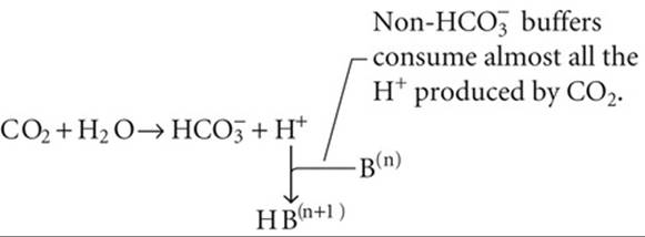
(28-28)

In this simplified approach, the final pH depends on two competing buffer reactions—one involving and the other involving HB⁽ⁿ⁺¹⁾/B⁽ⁿ⁾. Computing the final pH requires solving two simultaneous equations, one for each buffer reaction.

The Buffer

The first of the two equations that we must solve simultaneously is a rearrangement of the Henderson-Hasselbalch equation (see Equation 28-16):

(28-29)

For a of 40 mm Hg, the equation requires that [] be 24 mM when pH is 7.40—as in normal arterial blood plasma. If pH decreases by 0.3 at this same , Equation 28-29 states that [] must fall by half to 12 mM. Conversely, if pH increases by 0.3, [] must double to 48 mM. The blue column of Table 28-4 lists the [] values that Equation 28-29 predicts for various pH values when is 40 mm Hg. Plotting these [] values against pH yields the blue curve labeled “ = 40 mm Hg” in Figure 28-6A. This curve, which is known as a CO₂ isobar or isopleth (from the Greek isos [equal] + plethein [to be full]) represents all possible combinations of ] and pH at a of 40 mm Hg. Table 28-4 also summarizes [] values prevailing at values of 20 and 80 mm Hg. Note that at a of 20 (orange column), representing respiratory alkalosis, [] values are half those for a of 40 at the same pH. At a of 80 (green column), representing respiratory acidosis, [] values are twice those at a of 40. Each of the isopleths in Figure 28-6A rises exponentially with pH. The slope of each isopleth also rises exponentially with pH and represents β_open for . At a particular pH, an isopleth representing a higher (i.e., a higher []) has a steeper slope, as Equation 28-20 predicts.

TABLE 28-4

Relationship between and pH at Three Fixed Levels of

[] (mM)
pH	= 20 mm Hg	= 40 mm Hg	= 80 mm Hg
7.1	6 mM	12 mM	24 mM
7.2	8	15	30
7.3	10	19	38
7.4	12	24	48
7.5	15	30	60
7.6	19	38	76
7.7	24	48	96

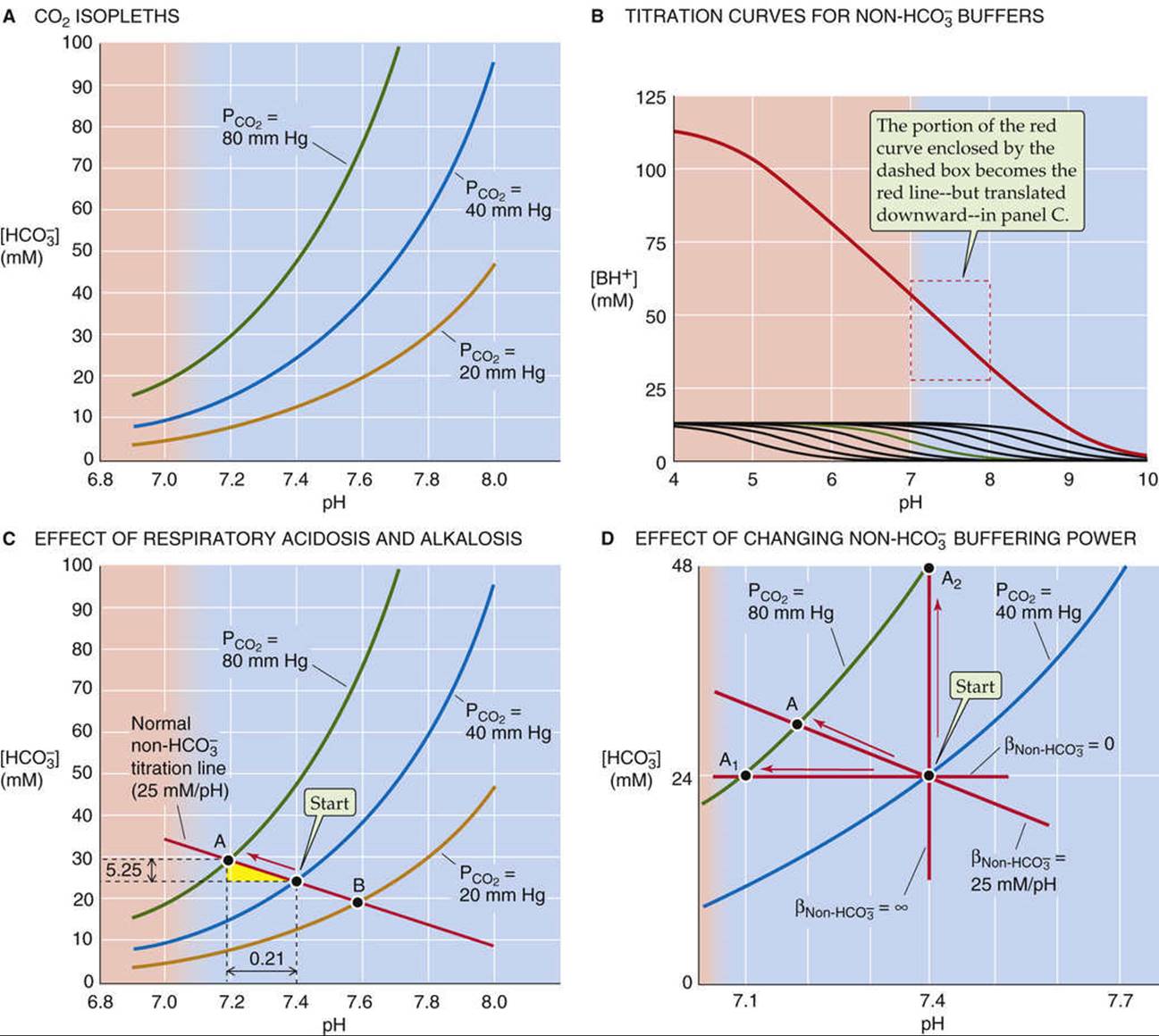
FIGURE 28-6 Davenport diagram. In A, the three isopleths are CO₂ titration curves. In B, the solution contains nine buffers, each at a concentration of 12.6 mM and with pK values evenly spaced 0.5 pH unit apart, as in Figure 28-2B. In C, the red arrow represents the transition from a normal acid-base status for blood (“Start”) to respiratory acidosis (point A) produced by raising to 80 mm Hg. Point B represents respiratory alkalosis produced by lowering to 20 mm Hg. In D, the labeled points represent the results of respiratory acidosis when is zero (point A₁), 25 mM/pH (point A), and infinity (point A₂).

Buffers

The second of the two equations that we must solve simultaneously describes the lumped reaction of all buffers. To understand the origin of this equation, we begin with the green curve (surrounded by black curves) in Figure 28-6B, the titration curve of a single buffer with a pK of 7 and total buffer concentration of 12.6 mM (as for the green curve in Fig. 28-2B). At a pH of 10, [HB⁽ⁿ⁺¹⁾] for this single buffer is extremely low because almost all of the “B” is in the form B⁽ⁿ⁾. As we lower pH by successively adding small amounts of HCl, [HB⁽ⁿ⁺¹⁾] gradually rises—most steeply when pH equals pK. Indeed, at any pH, the slope of this curve is the negative of β for this single buffer. The black curves in Figure 28-6B are the titration curves for eight other buffers, each present at a [TB] of 12.6 mM, with pK values evenly spaced at intervals of 0.5 pH unit on either side of 7. The red curve in Figure 28-6B is the sum of the titration curves for all nine buffers. N28-8 Its slope—the negative of the total buffering power of all nine buffers—is remarkably constant over a broad pH range. (The red curve in Figure 28-2B shows how β, the slope of the red curve here in Figure 28-6B, varies with pH.) The red curve in Figure 28-6B represents the second of the two equations that we must solve simultaneously.

N28-8

Davenport Diagram—Constructing the Buffer Line

Contributed by Emile Boulpaep, Walter Boron

The buffer line (the red line in Fig. 28-6B, C) describes the buffering power of all buffers other than (). In whole blood—here we refer to the line as the blood buffer line—hundreds of buffer groups may contribute to the overall buffering power. Each of these buffer groups has its own pK and concentration, and thus its own bell-shaped curve—like the nine small curves in Figure 28-2B—describing the pH dependence of its buffering power. Each of these buffer groups also has its own titration curve, as shown in Fig. 28-6B, and the sum of these titration curves (the red curve in this figure) is the combined titration curve of these buffers (i.e., ). Notice that this red curve is nearly a straight line over the physiological pH range. In other words, in the physiological range, the slope of the red line is nearly constant, which is another way of stating that the buffering power is nearly constant over this pH range—as illustrated in Figure 28-2B.

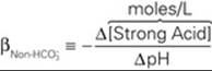
We already know from Equation 28-8 (reproduced below as Equation NE 28-21) that we can define buffering power in terms of the amount of strong acid added to the solution:

(NE 28-21)

From the perspective of the buffers that are at work during respiratory acidosis, Δ[strong acid] is the H⁺ formed from CO₂ and H₂O as a result of the increase in (see arrow from “Start” to point A in Fig. 28-6C). Because respiratory acidosis produces and H⁺ in a 1 : 1 ratio, the amount of formed during respiratory acidosis—that is —is the same as the amount of H⁺ added (Δ[strong acid]). Thus, we can replace Δ[strong acid] in Equation NE 28-21 with and therefore somewhat paradoxically express the buffering power in terms of []:

(NE 28-22)

and pH_init represent initial values (before increasing —that is, the point labeled “Start” in Fig. 28-6C), and [] and pH represent final values (after increasing —that is, point A in Fig. 28-6C). The equation describing the buffer line is simply a rearrangement of Equation NE 28-22:

(NE 28-23)

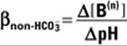
This equation describes a line whose slope is negative . For whole blood, is 25 mM/pH unit, so that the slope of the line is −25 mM/pH unit in Figure 28-6C. Note that because we assumed that the buffering power of the buffers is constant over the pH range of interest, and because this buffering power is represented by the slope of the buffer curve in Figure 28-6C, the function describing this buffering power must be a straight line (i.e., a function with a constant slope).

We are now in a position to understand why, in Figure 28-6C, the buffer line (see Equation NE 28-23) shares the same y-axis as the CO₂ isopleth (e.g., the blue curve in Fig. 28-6C), which is described by Equation 28-29, reproduced here:

(NE 28-24)

In both the case of the line describing the buffering power (see Equation NE 28-23) and the exponential curve describing the open-system CO₂ buffering power (see Equation NE 28-24), the dependent variable is [].

The buffer line passes through the point describing the initial conditions (pH_init, ). In Figure 28-6C, pH_init is 7.40 and is 24 mM, as indicated by the point labeled “Start.” Because these initial conditions for the buffers can change, we will see below in the text that the buffer line can translate up and down on the Davenport diagram in metabolic alkalosis and metabolic acidosis. However, as long as is constant, the slope of the line is always the same.

Solving the Problem

Figure 28-6C is a Davenport diagram, a combination of the three CO₂ isopleths in Figure 28-6A and the linear part of the red titration curve in Figure 28-6B. The red titration line (representing for whole blood, 25 mM/pH unit) intersects with the CO₂ isopleth for a of 40 at the point labeled “Start,” which represents the initial conditions for arterial blood. At this intersection, both and buffers are simultaneously in equilibrium.

We are now in a position to answer the question raised at the beginning of this section: What will be the final pH when we increase the of whole blood from 40 to 80 mm Hg? The final equilibrium conditions for this case of respiratory acidosis must be described by a point that lies simultaneously on the red titration line and the green isopleth for 80 mm Hg. Obtaining the answer using the Davenport diagram requires a three-step process:

Step 1: Identify the point at the intersection of the initial isopleth and the initial titration line (see Fig. 28-6C, “Start”).

Step 2: Identify the isopleth describing the final (80 mm Hg in this case).

Step 3: Follow the titration line to its intersection with the final isopleth. In Figure 28-6C, this intersection occurs at point A, which corresponds to a pH of 7.19 and an [] of 29.25 mM.

As discussed above, in the absence of buffers, this same doubling of causes a larger pH decrease, from 7.4 to 7.1.

By following three similar steps, we can use the Davenport diagram to predict the final pH and [] under conditions of a respiratory alkalosis. For example, what would be the effect of decreasing by half, from 40 to 20 mm Hg? In Figure 28-6C follow the red titration line from “Start” to its intersection with the orange isopleth for a of 20 mm Hg (point B), which corresponds to a pH of 7.60 and an [] of 19 mM. If the solution had not contained buffers, halving the would have caused a larger pH increase, from 7.4 to 7.7.

The amount of formed or consumed during “respiratory” acid-base disturbances increases with

Although it is reasonable to focus on CO₂ during respiratory acid-base disturbances, it would be wrong to assume that [] is constant. For example, in Figure 28-6C, where is 25 mM/pH unit, increasing from 40 to 80 mm Hg causes [] to increase from 24 to 29.25 mM. Thus, in each liter of solution, 5.25 mmol CO₂ combines with 5.25 mmol H₂O to form 5.25 mmol (which we see as the value between “Start” and point A) and 5.25 mmol H⁺. Nearly all of this H⁺ disappears as nearly 5.25 mmol of the deprotonated buffers (B⁽ⁿ⁾) consumes H⁺ to form nearly 5.25 mmol of their conjugate weak acids (HB⁽ⁿ⁺¹⁾). Thus, the flux through the reaction sequence in Equation 28-28 is nearly 5.25 mmol for each liter of solution.

(28-30)

Thus, the buffers drive the conversion of CO₂ to . These buffers minimize the increase in free [H⁺] that a given flux of CO₂ can produce. Thus, with a high , a large amount of CO₂must “flux” through Equation 28-30 before the free concentrations of and H⁺ rise sufficiently to satisfy the equilibrium (see Equation 28-14).

varies with the hemoglobin content of blood. Thus, patients with anemia have a low , whereas patients with polycythemia have a high .

Figure 28-6D illustrates the importance of . If is zero, the titration line is horizontal, and doubling from 40 to 80 mm Hg does not change [] significantly (see Fig. 28-6D, point A₁); this verifies our earlier conclusion (see Fig. 28-5, stage 3A). Simultaneously, pH falls by 0.3, which corresponds to a near-doubling of [H⁺]. Thus, doubling [CO₂] leads to a doubling of the product [][H⁺], so that the ratio [][H⁺]/[CO₂]—the equilibrium constant, K—is unchanged (Table 28-5, top row). Figure 28-6D also shows what happens if has the normal value of 25 mM/pH unit. Here, point A is the same as point A in Figure 28-6C, and it shows that [] increases by 5.25 mM, or 17% (see Table 28-5, middle row). Finally, if were ∞, the titration line would be vertical, and doubling would not change pH at all (point A₂ in Fig. 28-6D). In this case, [] would double, so that the doubling of the product [][H⁺] would match the doubling of (see Table 28-5, bottom row).

TABLE 28-5

Relationship between and the Amount of Formed in Response to a Doubling of

BUFFERING POWER	ΔpH	FORMED (mM)	FRACTIONAL Δ[H+]	FRACTIONAL	FRACTIONAL × Δ[H+]
0	−0.30	0.000,040	1.999,997	1.000,002	2.00
25	−0.21	5.25	1.71	1.17	2.00
∞	0	24.0	1.00	2.00	2.00

Adding or removing an acid or base—at a constant —produces a “metabolic” acid-base disturbance

Above, we examined the effect of adding HCl in the absence of other buffers (see Fig. 28-3). Predicting the pH change for such an acid-base disturbance was straightforward because the titration of to CO₂consumed all buffered H⁺. The situation is more complex when the solution also contains buffers (Fig. 28-7, stage 1). When we add 10 mmol of HCl to 1 L of solution, the open-system buffer pair neutralizes most of the added H⁺, buffers handle some, and a minute amount of added H⁺ remains free and lowers pH (see Fig. 28-7, stage 2A). Because the system is open, the CO₂ formed during buffering of the added H⁺ escapes to the atmosphere. If this buffering reaction were occurring in the blood, the newly formed CO₂ would escape first into the alveolar air, and then into the atmosphere.

FIGURE 28-7 Metabolic acidosis and alkalosis in the presence of buffers. The red arrows in the Davenport diagrams represent the transition to metabolic acidosis (point C) and metabolic alkalosis (point D). This example differs from Figure 28-3, in which the solution contained no buffers other than .

How much of the added H⁺ (Δ[strong acid] = 10 mM) follows each of the three pathways in this example of metabolic acidosis? Answering this question requires dealing with two competing equilibria, the and the buffering reactions. As for respiratory acid-base disturbances, we cannot precisely solve the equations governing metabolic acid-base disturbances. However, we can use the Davenport diagram on the left of Figure 28-7 to obtain a graphical estimate of the final pH and [] through a four-step process:

Step 1: Identify the point describing the initial conditions (see Fig. 28-7, “Start” in graph on left).

Step 2: Following the black arrow labeled “2,” move downward (in the direction of decreased []) by 10 mM—the concentration of added H⁺—to the point labeled with an asterisk. In this maneuver, we assume that the reaction + H⁺ → CO₂ + H₂O has initially consumed all of the added H⁺. Of course, if this were true, the reaction would be far out of equilibrium and the pH would not have changed at all. Also, the buffers would not have had a chance to participate in the buffering of H⁺.

Step 3: Through the asterisk, draw a line (see Fig. 28-7, black line in left graph) that is parallel to the titration line.

Step 4: Following the black arrow labeled “4,” move to the intersection of the new black line and the original isopleth. This intersection occurs at point C, which corresponds to a pH of 7.26 and an [] of 17.4 mM. This maneuver tracks the reaction CO₂ + H₂O → + H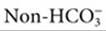⁺. buffers consume nearly all of this H⁺ in the reaction H⁺ + B⁽ⁿ⁾ → HB⁽ⁿ⁺¹⁾. As a result, [], [H⁺], and [HB⁽ⁿ⁺¹⁾] all rise and the system equilibrates.

As a shortcut, we could bypass the two black arrows and simply follow the red arrow along the CO₂ isopleth from “Start” to point C.

We now can return to the question of how much of the added H⁺ follows each of the three pathways in Figure 28-7, stage 2A. Because [] decreased by 24 − 17.4 = 6.6 mM, the amount of H⁺ buffered by must have been 6.6 mmol in each liter. Almost all of the remaining H⁺ that we added, nearly 3.6 mmol, must have been buffered by buffers. A tiny amount of the added H⁺, ~0.000,015 mmol, must have remained unbuffered and was responsible for decreasing pH from 7.40 to 7.26 (see Fig. 28-7, stage 3A).

Figure 28-7 also shows what would happen if we added 10 mmol of a strong base such as NaOH to our 1-L solution. The open-system buffer pair neutralizes most of the added OH⁻, buffers handle some, and a minute amount of added OH⁻ remains unbuffered, thus raising pH (see Fig. 28-7, stage 2B). The Davenport diagram on the right of Figure 28-7 shows how much of the added OH⁻follows each of the three pathways in this example of metabolic alkalosis. The approach is similar to the one we used above for metabolic acidosis, except that in this case, we generate a new black line that is displaced 10 mM above the titration line. We follow the isopleth to its intersection with this black line at point D, which corresponds to a final pH of 7.51 and an [] of 31.1 mM. Thus, [] rose by 31.1 − 24.0 = 7.1 mM. This is the amount of added OH⁻ that buffered. buffers must have buffered almost all of the remaining OH⁻ that we added, ~2.9 mmol in each liter. The unbuffered OH⁻, which was responsible for the pH increase, must have been in the nanomolar range (see Fig. 28-7, stage 3B, and Box 28-1).

Box 28-1

Strong Ion Difference

Some clinicians assess acid-base disorders in terms of a virtual parameter termed strong-ion difference (SID). Unlike weak acids and bases, the so-called strong cations and strong anions are fully dissociated at physiological pH. In blood,

Three major limitations to the SID approach are that (1) proteins and physiological processes generally depend on pH, not SID; (2) cells and the body closely regulate pH but have no known mechanism for directly sensing or regulating SID; and (3) SID neither is uniquely related to pH nor has a causal role in changing pH. Because the SID approach provides no new mechanistic insight, we focus on the classical pH/buffer approach.

During metabolic disturbances, makes a greater contribution to total buffering when pH and are high and when is low

In Figure 28-7, neutralized 7.1 mmol of the 10 mmol of OH⁻ added to 1 L (ΔpH = +0.11) but only 6.6 mmol of the added 10 mmol of H⁺ (ΔpH = −0.14). The reason for this difference is that the buffering power of in an open system increases exponentially with pH (see Fig. 28-4, blue curve). In the Davenport diagram, this pH dependence of β_open appears as the slope of the CO₂ isopleth, which increases exponentially with pH. Thus, adding alkali will always cause a smaller pH change than adding an equivalent amount of acid. In our example of metabolic alkalosis (see right side of Fig. 28-7), the mean β_open is (7.1 mM)/(0.11 pH unit) = 65 mM/pH unit in the pH range 7.40 to 7.51 (Table 28-6). On the other hand, in our example of metabolic acidosis (see left side of Fig. 28-7), the mean β_open is (6.6 mM)/(0.14 pH unit) = 47 mM/pH unit in the pH range 7.26 to 7.40, substantially less than in the more alkaline range. Because is 25 mM/pH unit over the entire pH range, β_total is greater in the alkaline pH range.

TABLE 28-6

Buffering Produced by and Buffers*

ADDITION	ΔpH			Δ[B(n)]		βtotal
+10 mmol H+	~ −0.14	~6.6 mM	47 mM/pH unit	~3.4 mM	25 mM/pH unit	72 mM/pH
+10 mmol OH−	~ +0.11	~7.1 mM	65 mM/pH unit	~2.9 mM	25 mM/pH unit	89 mM/pH

^*The additions are made to 1 L of solution. Initial pH = 7.40, = 40 mm Hg, = 24 mM. assumed to be 25 mM/pH unit.

We have already seen that β_open is proportional to [] (see Equation 28-20) and that—at a fixed pH—[] is proportional to (see Equation 28-29). Thus, other things being equal, the contribution of β_open to total buffering increases with . Patients with a high due to respiratory failure will, therefore, have a higher buffering power than normal individuals at the same pH.

Because and buffers compete for added OH⁻ or H⁺, the contribution of to total buffering also depends on . Figure 28-8 illustrates the effects of adding 10 mmol NaOH to our standard 1-L solution at values of 0, 25 mM/pH unit, and ∞. We saw in Figure 28-3, stage 3B, that adding 10 mmol of NaOH to a 1-L solution containing but no other buffers causes [] to increase from 24 to 34 mM, and pH to increase from 7.40 to 7.55. To use a Davenport diagram to solve the same problem (see Fig. 28-8A), we generate a titration line with slope of zero (because = 0) through the “Start” point. We also draw a black line with the same slope, but displaced 10 mM higher. Following the blue = 40 isopleth from “Start” to the point where the isopleth intersects with the black line at point D₁, we see that—as expected—the final pH is 7.55 and the final [] is 34 mM. Thus, must buffer virtually all 10 mmol of OH⁻ added to 1 L. Because the total buffering power is simply β_open, the pH increase must be rather large, 0.15.

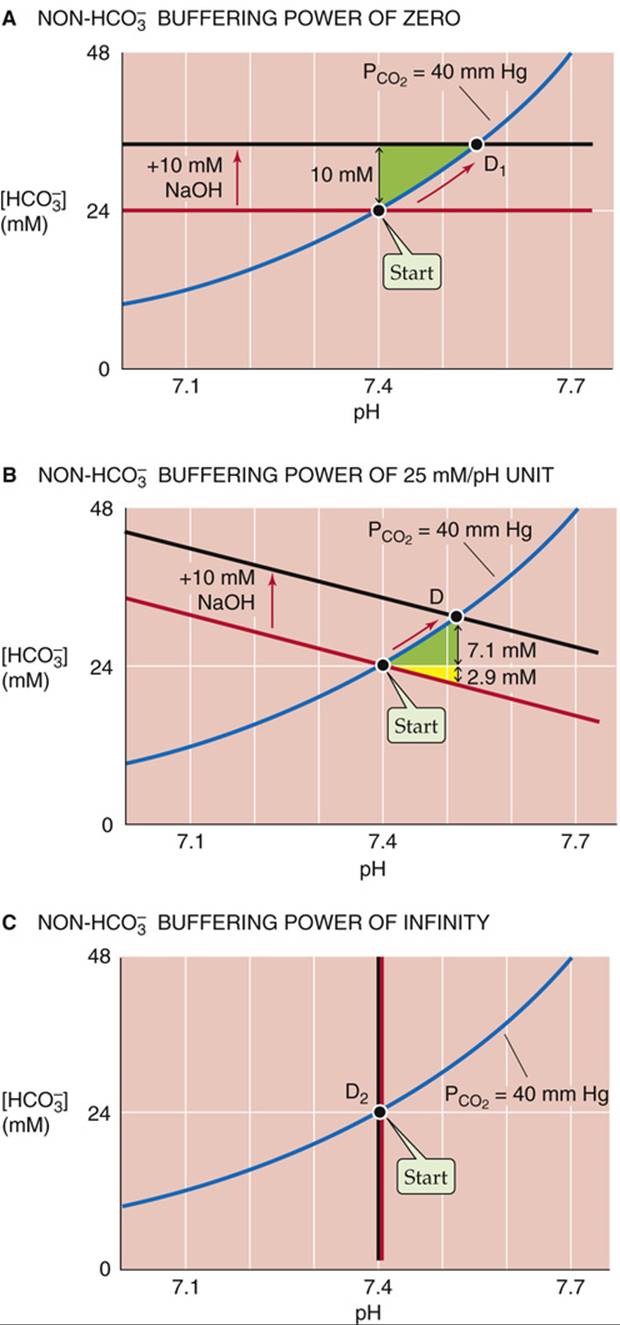
FIGURE 28-8 Effect of on the pH increase caused by metabolic alkalosis.

When is 25 mM/pH unit, as in the Davenport diagram in the upper right of Figure 28-7 (replotted in Fig. 28-8B), can buffer only 7.1 mmol because the buffers neutralize 2.9 mmol. With the increased total buffering power, the pH increase is only 0.11.

Finally, when is ∞, the black line lies right on top of the vertical titration line (see Fig. 28-8C). Thus, neither [] nor pH changes at all. However, [HB⁽ⁿ⁺¹⁾] increases by 10 mM because the infinitely powerful buffers do all of the buffering.

This set of three examples—for values of 0, 25, and ∞—is comparable to the set that we discussed above for respiratory acidosis in Figure 28-6D.

A metabolic change can compensate for a respiratory disturbance

Thus far, we have considered what happens during primary respiratory and metabolic acid-base disturbances. When challenged by such acid or alkaline loads in the blood plasma, the body compensates by altering [] or , returning pH toward its initial value and minimizing the magnitude of the overall pH change.

In Figure 28-9A we revisit an example, originally introduced in Figure 28-6C, in which we produced a primary respiratory acidosis by increasing from 40 to 80 mm Hg (red arrow in Fig. 28-9A between “Start” and point A at pH 7.19). If the high persists, the only way we can restore pH toward its initial value of 7.40 is to add an alkali (e.g., or OH⁻) or remove an acid (e.g., H⁺), all of which are equivalent. N28-9 Adding 10 mmol of OH⁻ to 1 L, for example, superimposes a metabolic alkalosis on the primary respiratory acidosis—a metabolic compensation to respiratory acidosis.

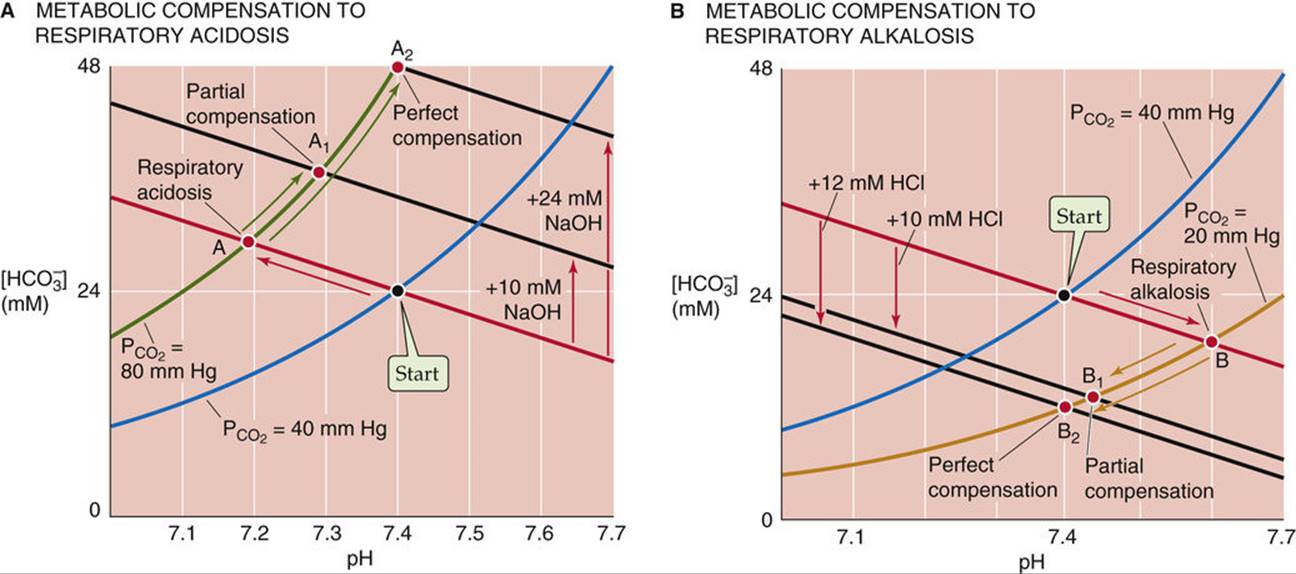
FIGURE 28-9 Metabolic compensation to primary respiratory acid-base disturbances.

The Davenport diagram predicts the consequences of adding 10 mmol of OH⁻ to 1 L. We start by generating a black line that is parallel to the red titration line, but displaced upward by 10 mM. Point A₁, the intersection of the black line and the isopleth for 80 mm Hg, represents a final pH of 7.29, still lower than the normal 7.40, but much higher than the 7.19 prevailing before compensation.

If we add an additional 14 mmol OH⁻, for a total addition of 24 mmol OH⁻ to 1 L, pH returns to exactly its initial value of 7.40 (point A₂ in Fig. 28-9A). In other words, we can perfectly compensate for doubling from 40 (“Start”) to 80 mm Hg (point A) by adding an amount of OH⁻ equivalent to the amount of that was present (i.e., 24 mM) at “Start.” Perfect compensation of respiratory acidosis is an example of isohydric hypercapnia (i.e., same pH at a higher ):

(28-31)

The kidneys are responsible for the metabolic compensation to a primary respiratory acidosis. They acutely sense high and may also chronically sense low blood pH. The response is to increase both the secretion of acid into the urine and the transport of into the blood (see pp. 832–833), thereby raising plasma pH—a compensatory metabolic alkalosis. The renal compensation to a substantial respiratory acidosis is not perfect, so that pH remains below the normal value of 7.40.

The kidneys can also perform a metabolic compensation to a respiratory alkalosis. In Figure 28-9B we revisit a second example, originally introduced in Figure 28-6C, in which we produced a primary respiratory alkalosis by decreasing from 40 to 20 mm Hg (red arrow in Fig. 28-9B between “Start” and point B at pH 7.60). We can compensate for most of this respiratory alkalosis by adding 10 mmol of H⁺to each liter of solution or by removing 10 mmol NaHCO₃ or NaOH, all of which produce the same effect. We generate a black line that is parallel to the red titration line but is displaced downward by 10 mM. Point B₁ (pH 7.44), at the intersection of the black line and the isopleth for 20 mm Hg, represents a partial compensation.

If we add an additional 2 mmol H⁺, for a total addition of 12 mmol of H⁺ to each liter, pH returns to exactly its initial value of 7.40 (point B₂ in Fig. 28-9B). Why is this amount so much less than the 24 mmol of OH⁻ that we added to each liter to compensate perfectly for a doubling of ? When we halve , we need only add an amount of H⁺ equivalent to half the amount of that was present (24/2 = 12 mM) at “Start.”

In response to a primary respiratory alkalosis, the kidneys secrete less acid into the urine and transport less into the blood (see pp. 833–834), thereby lowering plasma pH—a compensatory metabolic acidosis.

A respiratory change can compensate for a metabolic disturbance

Just as metabolic changes can compensate for respiratory disturbances, respiratory changes can compensate for metabolic ones. In Figure 28-10A we return to an example originally introduced on the left side of Figure 28-7, in which we produced a primary metabolic acidosis by adding 10 mmol of HCl to 1 L of arterial blood (red arrow in Fig. 28-10A between “Start” and point C at pH 7.26). Other than removing the H⁺(or adding OH⁻ to neutralize the H⁺), the only way we can restore pH toward the initial value of 7.40 is to lower . That is, we can superimpose a respiratory alkalosis on the primary metabolic acidosis—a respiratory compensation to a metabolic acidosis. For example, we can compensate for most of the metabolic acidosis by reducing from 40 to 30 mm Hg. Starting at C, follow the black line from the isopleth for 40 mm Hg to the new isopleth for 30 mm Hg at point C₁ (pH 7.34). This maneuver represents a partial compensation.

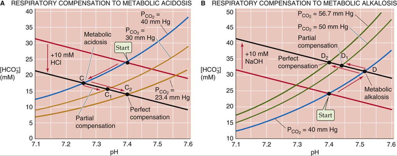
FIGURE 28-10 Respiratory compensation to primary metabolic acid-base disturbances.

If we reduce by an additional 6.6 mm Hg to 23.4 mm Hg, we produce a perfect compensation, which we represent in Figure 28-10A by following the black line from C until we reach pH 7.40 at point C₂, which is on the isopleth for 23.4 mm Hg. Perfect compensation requires that we reduce by a fraction (i.e., [40 − 23.4]/40 ≅ 0.42) that is identical to the ratio of added HCl to the original [] (i.e., 10/24 ≅ 0.42).

Not surprisingly, the respiratory system is responsible for the respiratory compensation to a primary metabolic acidosis. The low plasma pH or [] stimulates the peripheral chemoreceptors (see p. 710) and, if sufficiently long-standing, also the central chemoreceptors (see pp. 713–715). The result is an increase in alveolar ventilation, which lowers (see pp. 679–680) and thus provides the respiratory compensation.

The body achieves a respiratory compensation to a primary metabolic alkalosis in just the opposite manner. In Figure 28-10B, we revisit an example originally presented on the right side of Figure 28-7, in which we produce a primary metabolic alkalosis by adding 10 mmol of NaOH to 1 L (red arrow in Fig. 28-10B between “Start” and point D at pH 7.51). If we now increase from 40 to 50 mm Hg, we partially compensate for the metabolic alkalosis by moving from D to D₁ (pH 7.44). If we raise by an additional 6.7 mm Hg to ~56.7 mm Hg, the compensation is perfect, and pH returns to 7.40 (D₂).

In response to a primary metabolic alkalosis, the respiratory system decreases alveolar ventilation and thereby raises . The compensatory respiratory acidosis is the least “perfect” of the four types of compensation we have discussed. The reason is that one can decrease alveolar ventilation—and thus oxygenation—only so far before compromising one's very existence.

In a real person, each of the four primary acid-base disturbances—points A, B, C, and D in Figures 28-9 and 28-10—occurs in the extracellular fluid. In each case, the body's first and almost instantaneous response is to use extracellular buffers to neutralize part of the acid or alkaline load. In addition, cells rapidly take up some of the acid or alkaline load and thus participate in the buffering, as discussed below. Furthermore, renal tubule cells may respond to a metabolic acidosis of extrarenal origin (e.g., diabetic ketoacidosis) by increasing acid secretion into the urine, or to a metabolic alkalosis (e.g., NaHCO₃ therapy) by decreasing acid secretion—examples of metabolic compensation to a metabolic disturbance. Points C and D in Figure 28-10 include the effects of the actual acid or alkaline load, extracellular and intracellular buffering, and any renal (i.e., “metabolic”) response.

Position on a Davenport diagram defines the nature of an acid-base disturbance

The only tools needed for characterizing acid-base status (i.e., pH, [], and ) are a Davenport diagram and electrodes for measuring pH and . From these last two parameters, we can compute [] using the Henderson-Hasselbalch equation. The acid-base status of blood plasma—or of any aqueous solution—must fall into one of five major categories:

1. Normal. For arterial blood, pH is 7.40, [] is 24 mM, and is 40 mm Hg. This point was labeled “Start” in the previous figures and is the central point in Figure 28-11A through D.

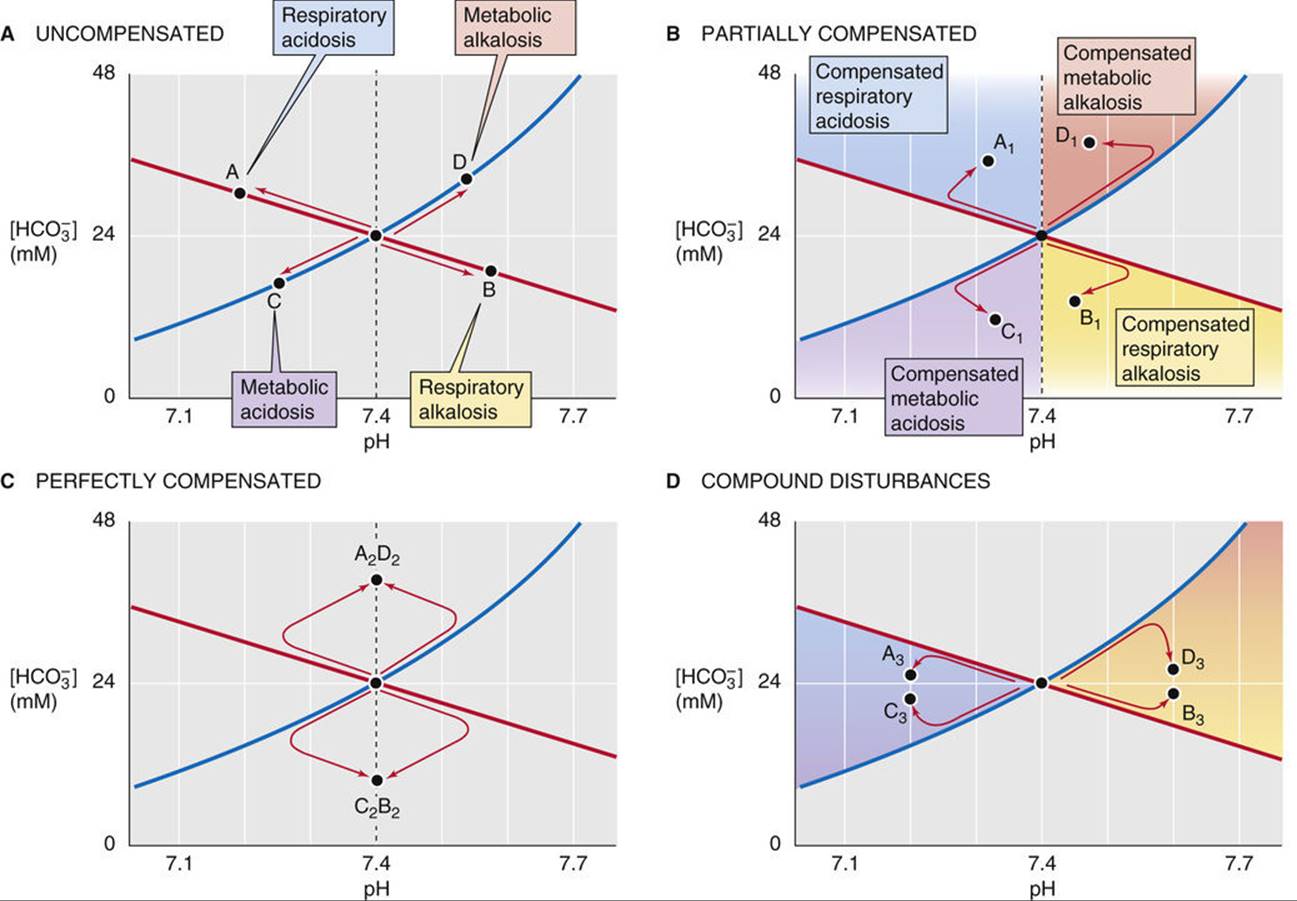
FIGURE 28-11 Acid-base states represented by position on a Davenport diagram.

2. One of the four primary (or uncompensated) acid-base disturbances. The coordinates for pH and [] fall either (a) on the titration line, but off the 40-mm Hg isopleth for uncompensated respiratory acidosis (point A, Fig. 28-11A) or alkalosis (point B); or (b) on the 40-mm Hg isopleth, but off the titration line for an uncompensated metabolic acidosis (point C) or alkalosis (point D).

3. A partially compensated disturbance. The coordinates for pH and [] fall in any of the four colored regions of Figure 28-11B. For example, point A₁ in the blue region represents a partially compensated respiratory acidosis. In a subject for whom a respiratory acidosis has existed for longer than a few hours, increased renal H⁺ excretion has probably already begun producing a metabolic compensation. Depending on the extent of the original acidosis and the degree of compensation, point A₁ could lie anywhere in the blue region. We can reach similar conclusions for the other three disturbances/compensations.

4. A perfectly compensated disturbance. The point falls on the vertical line through pH 7.4. As indicated by point A₂D₂ in Figure 28-11C, a perfect compensation following respiratory acidosis is indistinguishable from that following metabolic alkalosis. In either case, the final outcome is isohydric hypercapnia. Similarly, point B₂C₂ represents a perfect compensation following either metabolic acidosis or respiratory alkalosis (isohydric hypocapnia).

5. A compound respiratory/metabolic disturbance. The point falls in one of the two colored regions in Figure 28-11D. For example, points A₃ and C₃ represent a respiratory acidosis complicated by metabolic acidosis, and vice versa. The second disturbance causes the pH to move even further away from “normal,” as might occur in an individual with both respiratory and renal failure (see Table 28-3). Of course, it is impossible to determine if one of the two compounding disturbances developed before the other.