STUDY HINTS
A large part of genetic analysis depends upon accurate statistical treatment of data. As we have pointed out earlier, probabilities help form the hypotheses against which patterns of inheritance and gene action can be tested. The same is true of quantitative genetics. In this instance, however, the patterns are complicated by the fact that one is dealing not only with the segregation of several genes but also with environmental factors that can mask the expression of alleles in the genotype. Several important genetic specialties, such as biometrical genetics, are concerned with ways of extracting information about the genotype from quantitative phenotypes.
Perhaps the most commonly used measures of quantitative distributions are the mean, standard deviation, variance, and standard error. These measures are described briefly in the following table (and in the Glossary).
|
Measure |
Symbol |
Calculation |
|
Mean |
|
The sum of all individual measurements divided by the sample size (n) |
|
Standard deviation |
s, s.d., or σ |
|
|
Variance |
s2σ2, |
|
|
Standard error |
s.e. or S |
|
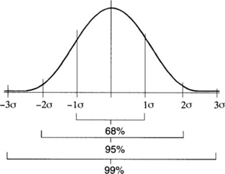
Using these measurements of mean and of dispersal around the mean, one can accurately describe many aspects of a quantitative distribution. Of these, perhaps the standard deviation is the most useful statistically. Predictable proportions of the population of values will fall within one, two, or three standard deviations of the mean. These are shown precisely in some texts, but for convenience the divisions are often rounded off as illustrated in the figure at left.
Since quantitative phenotypic distributions, such as those for height or IQ, involve both genetic segregation and environmental influences, it is useful to have ways of predicting the relative importance of each of these factors for a given trait or population. Although gene number can only be estimated crudely, consider the expectations based on simple Mendelian segregation. If one pair of alleles is segregating, 1/4 of the F2 progeny should be as extreme in phenotype as each of the original parents (e.g., 1/4 should be as short as the shorter parent and 1/4 as tall as the taller parent in an original cross between short and tall). When two pairs of alleles contribute to the trait, 1/16, or (1/4)2, of the F2 progeny are as extreme as each of the original parental phenotypes. Generalizing from this, (1/4)n of the F2 progeny should be in this extrene class, where n is the number of loci segregating in the cross.
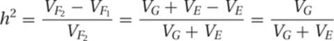
In a more general way, we can ask what proportion of the total phenotypic variance is due to genetic causes. This proportion of heritable variance is called heritability and is symbolized h2 (the squared term simply indicates that it is derived from variances). In the most restricted or narrow sense, the estimated genetic effects are limited to additive genetic segregation. In the broad sense, heritability reflects gene interactions, variations in dominance, and other genetic complications. The heritability resulting from additive segregation is the most important type for predicting the response of a population to selection or patterns of transmission. We will therefore limit our discussion to heritability in the narrow sense.
Calculations of heritability can be done in a number of ways, such as by measuring the regression of offspring phenotypes on parent phenotypes or by comparing the variances in generations bred from crosses between homozygous strains. We can illustrate the logic of such measurements by considering the sources of variation in the F1 and F2 generations produced by crossing inbred parental lines.
All variation is environmental
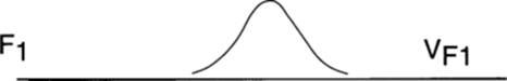
The individuals in the distribution are genetically the same; all variation (V) is environmental (VE), since all individuals are homozygous for alleles they share, and all are heterozygous for alleles that differ between the parental strains.
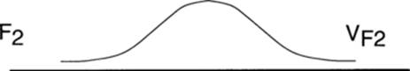
Variation is the result of both environmental factors (VE) and genetic segregation (VG).
Thus one way to calculate heritability is as follows:
When evaluating distributions, we frequently would like to know how different they are from each other. The t test is a statistical test that allows us to calculate the significance of the difference between two means. It takes into account the variances (![]() and
and ![]() ) and the sample sizes (n1 and n2) of each distribution.
) and the sample sizes (n1 and n2) of each distribution.
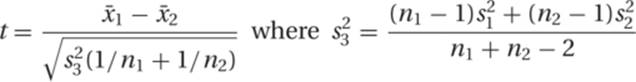
In a t test, the null hypothesis is that the two distributions are samples from the same population of measurements; that is, the two distributions are not significantly different. The use of a null hypothesis comes from a consideration of the limitations of information and the structure of logic. It is a sort of default position. Consider, for example, the statement “All genetics students know a person named Richard.” This statement is difficult (or even impossible) to prove correct, since it would involve surveying every known student of genetics, but it is easy to disprove. All one needs to do is find one example of a student who does not know someone named Richard. The null hypothesis in a statistical test works the same way. One cannot readily prove an idea, but one can disprove it, or at least establish strong evidence against it. In a t test and similar tests used in quantitative genetics, the formulation of the appropriate null hypothesis is very important. Usually, the null hypothesis is that the two things or sets being compared are the same. One can readily marshal evidence to support the idea that they are different, so one ends up approaching the problem backward. By failing to disprove the null hypothesis, one indirectly supports the alternative.
IMPORTANT TERMS
Analysis of variance
Class intervals
Coefficient of variation
Correlation
Covariance
Frequency distribution
Heritability
Multiple-factor inheritance
Null hypothesis
Polygene
Population
Quantitative characters
Regression
Standard deviation
Standard error
Statistics
t test
Variance
PROBLEM SET 9
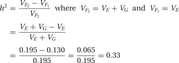
1. In a hypothetical experiment, we cross two strains of chickens that are genetically different with respect to several gene loci that affect egg weight. We discover that the F2 variance in egg weight is .195, but the F1 variance is only .130. From this we can conclude that the heritability for egg weight in these chickens is about
(a) .66,
(b) .20,
(c) .33,
(d) .13,
(e) none of the above.
link to answer
2. In the F2 generation of a cross between tall snapdragons and short snapdragons, a total of 30 plants (of 7,678 plants measured) were as short as the original short snapdragon parental strain. From these data, please estimate the number of segregating loci affecting plant height in this cross.
link to answer
3. In a random sample of 100,000 fifth-graders, the average IQ was found to be 100, and the standard deviation was 15 IQ points.
(a) What number of students would be expected to have an IQ over 130?
(b) How many would have an IQ between 70 and 100?
(c) How many would have an IQ within one standard deviation of the mean?
link to answer
4. Assume an animal population has just one segregating locus on each of its 20 pairs of chromosomes, and assume that each locus has 3 alleles (chromosome 1 has alleles A1, A2, or A3; chromosome 2 has alleles B1, B2, or B3, and so forth). What is the number of genetically different gametes that such an animal can produce?
link to answer
5. For the animal population described in problem 4, how many different genotypes are possible?
link to answer
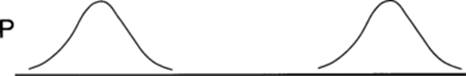
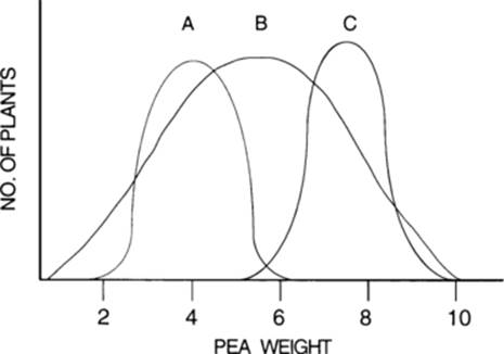
6. Assume that three strains of garden peas (A, B, and C) produce the samples of peas indicated in the accompanying figure. All three samples contain the same number of individuals and come from plants raised in the same environment. The strain that is the most inbred is probably
(a) A,
(b) B,
(c) C.
link to answer
7. Assume that a pure-breeding plant with red flowers is crossed with a pure-breeding plant with white flowers and that flower color is a polygenic trait, with the two parent strains differing at seven loci. The F1 will all be intermediate in flower color. In the F2, about one plant in how many will be expected to have white flowers?
(a) 8,
(b) 16,
(c) 32,
(d) 64,
(e) 4,000,
(f) 16,000,
(g) 64,000,
(h) 256,000.
link to answer
8. Plant populations A and B each have a mean height of 1.8 meters, with a standard deviation of 0.3 meter in each case. Population A contains 50 plants, and population B consists of 100 plants. The standard error (standard deviation of the means) of population A will be
(a) the same as that of population B,
(b) larger than that of population B,
(c) smaller than that of population B.
link to answer
9. A sample of animals has a mean weight of 250 kilograms (kg) and a variance of 100. With this information we can predict that 34 percent of the animals will have weights ranging from
(a) 150 to 350 kg,
(b) 240 to 250 kg,
(c) 150 to 250 kg,
(d) 240 to 260 kg.
link to answer
10. The idealized, or classical, model of polygenic inheritance predicts a normal F2 distribution for various traits (such as height). On the other hand, if some of the loci had a dominant allele for increased height, what would the distribution look like?
link to answer
11. Calculate the mean, variance, and standard deviation for each of the following sets of data obtained by measuring bristle numbers on the fruit fly Drosophila melanogaster.
Data set 1: 12, 10, 5, 21, 8, 14, 18, 9, 18, 7
Data set 2: 19, 21, 16, 19, 20, 17, 22, 14, 18, 15
link to answer
12. Using a t test, determine whether the two sets of data given in problem 11 are consistent with the hypothesis that they came from the same population of Drosophila.
link to answer
13. Which of the following sets of data has the largest variance?
|
Mean |
Sample size |
Standard error |
|
|
1 |
19.348 |
25 |
0.9282 |
|
2 |
0.400 |
25 |
0.0494 |
|
3 |
113.375 |
16 |
0.9215 |
link to answer
14. The following data were obtained by measuring the lengths of new growth in two plots of a plant species maintained in different light–dark cycles. Is there a significant difference in the response to lighting conditions?
Sample 1: 25.5, 19.7, 16.5, 23.6, 21.3, 12.2, 16.8, 14.5, 27.4, 16.0
Sample 2: 16.7, 22.1, 28.3, 12.1, 24.8, 25.4, 16.8, 15.5, 22.0, 18.9
link to answer
15. In which one or more of the following traits is genetic variance more influential than environmental factors in determining the phenotype? (Heritability estimates were obtained from D. S. Falconer, Introduction to Quantitative Genetics [London: Oliver & Boyd, 1960]).
|
Trait |
Heritability |
|
Milk production in cattle |
0.60 |
|
Litter size in pigs |
0.30 |
|
Egg production in poultry |
0.20 |
|
Puberty age in rats |
0.15 |
|
Wool length in sheep |
0.55 |
|
Amount of spotting in Friesian cattle |
0.95 |
|
Body weight in sheep |
0.35 |
|
Abdominal bristle number of Drosophila |
0.50 |
link to answer
ANSWERS TO PROBLEM SET 9
1.
(c) Heritability is defined as the proportion of phenotypic variance that is the result of genetic segregation. It can be calculated from the F1 variance (which is totally environmental, VE) and the F2 variance (which is composed of both environmental and genetic components, VG).
2. The number of segregating loci is estimated from the proportion of F2 offspring that are phenotypically like one of the original P generation parents (that is, are as extreme as one of the original extreme parental strains). For example, if there is only one locus segregating (A and a), then in the F2 a total of 1/4 of the progeny will be aa, like one (phenotypically extreme) original parent. Thus gene number can be estimated by reducing the observed data to the form (1/4)n where n is the number of segregating loci. In this problem 30/7,678 is almost exactly (1/4)4. There are therefore four segregating loci estimated from this evidence. Two important assumptions of this model are that
(a) there are only two alleles per locus and
(b) they are assorting independently. Unless there is evidence to the contrary, these assumptions should be made when evaluating one of our problems.
3.
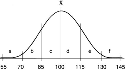
This figure shows the IQ distribution, with a mean of 100 and a standard deviation of 15. Standard deviations are marked to the left and right of the mean. Each region under the curve has been given a letter for convenience in discussing this problem.
(a) What proportion of students would be expected to have an IQ of over 130? Since 130 is 2 standard deviations above the mean, 95 percent of the population would have an IQ between 70 and 130 (sections b, c, d, e). Half of the remainder would have an IQ above 130 (section f). This is half of 5 percent, or 2.5 percent, which is 2,500 individuals from our sample.
(b) How many would have an IQ between 70 and 100? A total of 95 percent of the population falls within 2 standard deviations of the mean. Thus, half of 95 percent would have an IQ in the range 70–100 (sections b + c). This is 47,500 individuals.
(c) How many would have an IQ within 1 standard deviation of the mean? A total of 68 percent of the population has a phenotype within 1 standard deviation of the mean (an IQ in the range 85–115; sections c + d). This would involve 68,000 fifth-graders in our sample population.
4. For each of the 20 chromosomes there are three possibilities (allele 1, 2, or 3), independent of the genotypes of the other 19 chromosomes. The answer is therefore (3)20 = 3,486,784,401.
5. For each of the 20 loci there are n(n + 1)/2 combinations = 3(3 + 1)/2 = 6 different genotypes possible (A1A1, A2A2, A3A3, A1A2, A1A3, and A2A3). The answer is thus (6)20, which is 3,656,158,440,062,976. This large number is achieved with only 20 independently assorting loci, each with only 3 alleles, a striking demonstration of the ability of sexual reproduction, with its accompanying segregation and independent assortment, to generate hereditary variability.
6.
(c) Inbreeding increases the proportion of homozygotes and thus decreases the variance of the phenotype. The strain with the smallest variance, and therefore probably the most inbreeding, is C.
7.
(f) The proportion that will be as extreme as one original parental line is (1/4)n where n is the number of segregating loci. In this situation, (1/4)7 = 1/16,384. The closest answer is 16,000.
8.
(b) The standard error is defined as the standard deviation divided by the square root of the sample size (n). As n increases, the standard error decreases. Thus population A (where n = 50) will have a larger standard error than will population B (n = 100).
9.
(b) Since 34 percent is 1 standard deviation either above or below the mean, the only range that fits is 240–250 kg. Remember that the standard deviation is the square root of the variance. If you chose an answer such as (c), 150–250 kg, you may have done so because you did not read the question carefully enough to evaluate which statistics you were given to work with. This is a common error in working problems in genetics, but it is also an easy error to avoid. Remember, it is less painful to learn the lesson in a problem set like this than on a graded examination.
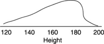
10. If polygenic alleles showed dominance, rather than being additive as they are commonly modeled, the distribution would be skewed toward increased height, as in the figure at left.
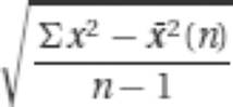
11. The equations for these parameters were given in the Study Hints for this chapter. For data set 1, the mean is 12.2, the variance is 28.844, and the standard deviation is 5.371. For data set 2, the mean is 18.1, the variance is 6.767, and the standard deviation is 2.601. If your calculations are similar to, but not exactly the same as, the ones we have given, it might simply be due to differences in the way in which the calculations are rounded at each step.
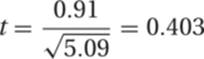
12. The null hypothesis for a t test is that the two samples come from the same population. A significantly large difference (i.e., large t-value) between the two sets of samples is evidence against the null hypothesis. To evaluate the similarity of this pair of samples, we substitute the following values into the equation for t given in the Study Hints:
From this we find that
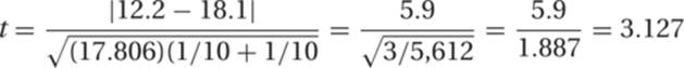
The number of degrees of freedom is n1 + n2 − 2 = 18. Using the reference table of t values (Table R.2), we find that for this magnitude of t and 18 degrees of freedom, p is between .01 and .001. This means that if one took two samples from the same population, one would expect to observe deviations this large or larger by chance alone with a frequency of between once in 100 and once in 1,000 times. This is clearly not likely, and one can interpret this as evidence against the hypothesis that the two data sets are from the same population.
13. The purpose of this question is to test your understanding of the relationships among the various measurements of a distribution. The standard error (s.e.) is the standard deviation (s.d. or s) divided by the square root of the sample size (n). This can be rearranged as
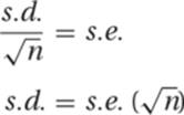
Substituting from the first set of data,
![]()
The variance is the square of the standard deviation, so in this case the variance equals 21.539. Your answer might be slightly different if you did not round off in the same way. Variances for the two remaining data sets are 0.061 and 13.587, respectively. Therefore, sample 1 has the largest variance.
14. The mean and variance for sample 1 are 19.35 and 25.012, whereas for sample 2 they are 20.26 and 25.980; n = 10 in both samples. Substituting into the formula for t,

Thus,
The number of degrees of freedom is n1 + n2 − 2 = 18 in this problem. From Table R.2 it can be seen that a t value this large or larger would occur frequently by chance alone. There is therefore no statistically significant difference between these samples.
15. Heritability is the proportion of total phenotypic variance that can be accounted for by genetic factors. Thus genetic influences are greater than environmental ones for traits in which h2 is greater than 0.5. This is true of milk production in cattle, length of wool in sheep, and amount of spotting in Friesian cattle. Abdominal bristle number in Drosophila apparently has equal genetic and environmental influences in this sample of heritabilities.
CROSSWORD PUZZLE 9
Quantitative Inheritance
Across
1. Inheritance in which several genes influence the phenotype of one quantitative character
6. Proportion of phenotypic variation in a given trait in a specified population that is accounted for by genetic segregation
8. Hypothesis that assumes that two samples are drawn from the same population or that a sample fits a specific model
9. Traits in which the phenotype is measured on a continuous scale
10. When two or more characteristics are dependent on, and vary with, each other
12. Measure of the extent to which values within a distribution depart from the mean
14. Values computed from sample data
15. Gene with a small effect that is involved in determination of a quantitative trait’s phenotype
16. Sum of all values, divided by the total number of data points
Down
2. Subdivisions made in frequency distributions to facilitate presentation and analysis
3. Group of individuals of the same species, in a defined area
4. Square root of the variance of the mean.
5. Distribution that arranges statistical data by demonstrating the number of occurrences of each value in a data set
7. Square root of the variance
11. Statistical method that will predict one character by using another that is correlated
13. Statistical test used to compare the differences between two distributions
 , where
 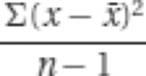 , square of the standard deviation