Bengt Källén1
(1)
Tornblad Institute, Lund University, Lund, Sweden
9.1 Risk Estimates
In order to epidemiologically investigate if an exposure (e.g., maternal use of a drug) causes an outcome (e.g., infant congenital malformations), one first has to look for an association between the two; if the outcome occurs more often than expected after the exposure. If so, the next step is to see if it is likely that the excess probably is random or if it is “statistically significant.”
The crucial point is then to determine the number of outcomes after the exposure and to get an estimate of how many one would have had if the exposure had not affected the outcome, that is, the expectednumber. You sometimes hear that you don’t expect a baby to be malformed (which is true), but “expected” here means what number you would expect if the exposure had no effect. The expected number has to be estimated from some sort of a control material, for instance, from the occurrence of the malformation in non-exposed infants.
If the observed number of outcomes exceeds the expected number, this indicates the presence of a risk associated with the exposure. In order to quantify this risk, one can use a risk ratio, that is, the ratio between the risk after exposure divided with the risk after non-exposure. We can go back to the simple 2 × 2 table shown already in the introduction. It consists of four central cells and the rand sums (totals).
|
Outcome |
No outcome |
Total |
|
|
Exposed |
N1 |
N2 |
N1 + N2 |
|
Unexposed |
N3 |
N4 |
N3 + N4 |
|
Total |
N1 + N3 |
N2 + N4 |
N1 + N2 + N3 + N4 |
The risk after exposure is thus N1/(N1 + N2) and after non-exposure N3/(N3 + N4) where N’s represent numbers in each cell and the risk ratio will be N1/(N1 + N2) divided by N3/(N3 + N4). If the risk ratio = 1, the risks are identical, and the exposure has no effect – if it is over 1, the exposure may increase the risk of outcome; if it is lower than 1, the exposure may protect against the outcome. Note thus that at null risk, the risk ratio estimate is 1.0, not 0.
The expected number in the “exposed, outcome” cell will be a product of the number of exposed infants and the risk in the total material, thus (N1 + N2)*(N1 + N3)/(N1 + N2 + N3 + N4).
Such risk estimates are difficult or impossible to calculate from case-control studies as the proportion between outcome and no outcome is already defined, for instance, two controls for each case.
The odds for exposure in the outcome is N1/N3 and in the non-outcome N2/N4 and the odds ratio is (N1/N3)/(N2/N4). Note that this will be the same if one instead divides the odds for outcome in the exposed with the odds for outcome in the non-exposed.
The odds ratio will with necessity always be larger than the risk ratio (because you divide with a smaller number), but when outcomes are relatively rare (like congenital malformations) and exposures are relatively rare (like most drug use), the difference between the odds ratio and the risk ratio will be small.
In cohort studies one can calculate both odds and risk ratios but in order to get a similar measure as that used in case-control studies, often odds ratios are used even though risk ratios would be more logical.
A risk ratio of 1.7 thus means that after exposure, the outcome is 70 % more common than without exposure. One should not mix this up with the absolute risk – the risk a woman who has taken a drug in early pregnancy has to get a malformed baby, for instance. If we say that the general risk to have a baby with a major malformation is 3 %, the 70 % risk increase means that the risk increases to 5.1 %. If we are talking about a spina bifida, where the risk in an unexposed fetus is perhaps 1/2000 (=0.0005), the 70 % risk increase will mean an absolute risk of 1/1176 (=0.0005*1.7). Moderate risk increases are usually of limited interest for the individual, but if the exposure is common in the population, they can cause a substantial number of damaged outcomes.
9.2 Is the Odds Ratio or Risk Ratio Statistically Significant?
Let us start with a simple situation where no adjustments are made, but we have a simple 2 × 2 table as shown above. We can take a hypothetical example of maternal use of a drug and the risk to have an infant with a cardiovascular defect. We have collected data for 1000 drug users and compared them with 1000 nondrug users. Among the latter, 1 % had a cardiovascular defect; among the former, 2 % had such a defect – the risk ratio is thus 2.0. The distribution of the numbers is seen in the table below.
|
Malformation |
No malformation |
Total |
|
|
Drug use |
20 |
980 |
1000 |
|
No drug use |
10 |
990 |
1000 |
|
Total |
30 |
1970 |
2000 |
The odds ratio is thus 20/980 divided by 10/990 = 2.02, very close to the risk ratio of 2.0. But is the difference certain or could it be random? To answer this, one can apply a chi-square test. If this is done, you will find that the chi-square is 3.38 which corresponds to a probability (p-value) of 0.07. If we have decided that we accept statistical significance if p < 0.05, the answer is thus: no, this can be a chance finding.
The chi-square test compares the observed and expected numbers in each of the four central cells in the 2 × 2 table and is based on a squared normal distribution.
In this calculation we have made the assumption that the cardiac defect rate after drug use could be either higher or lower than after no drug use, what is called a two-sided test. If we are absolute sure that the use of the drug cannot protect against getting an infant with a cardiovascular defect, then one can apply a one-sided test and then p = 0.03, thus statistically significant. It is customary to always use two-sided tests, but it is sometimes useful to consider what happens if you apply a one-sided test. There are actually situations when the use of a drug is associated with a lower than expected malformation risk, e.g., use of antihistamines at NVP – not because the drug protects against malformation but because NVP is associated with a well-functioning placenta and therefore with a slightly decreased risk for malformation. Therefore, drugs used for NVP may actually show a reduced risk.
The chi-square test is built on normal distributions, and when numbers are low, such approximations are not allowed. One can then use an exact test, Fisher test. If one applies this on the example above, the exact two-sided p-value is 0.10, thus slightly weaker than that calculated with the chi-square test (0.07). If we instead had 4 malformed infants in the exposed group and 2 in the non-exposed group (which would give the same risk ratio), the chi-square test would give p = 0.41 and the Fisher test p = 0.68 – with so few cases, only the Fisher test should be used. As a rule of thumb, when the expected number in the smallest cell is less than 10, chi-square tests should be replaced by exact tests.
The importance of the p-value should be looked upon with some light-heartedness. A significant p-value does not necessarily prove that the association is true. A p-value of 0.04 (which is thus significant according to the most commonly used definition) only means that the chance that the finding is random is 1 in 25, comparable to the chance to draw a red king from a pack of cards on the first trial, which of course may happen and does not prove that you are an unusually clever finder of a red king. An association which is not statistically significant may well be true but the data so far do not show that they are, and it does not prove that no association exists. The difference between a p-value = 0.049 and one = 0.051 is not very large, but the former is regarded as significant, but not the latter. We will come back to this later in the text.
This may also be the place to point out the difference between a statistically significant effect and a clinically significant effect. The latter has two aspects: the significance for the individual case and the significance for the occurrence of the outcome in the population. If there is a moderate increase (say, a 50 % increase) of a common malformation (say a cleft lip/palate), this is of little importance for the individual which has been exposed. If the unexposed infant has a risk of such a defect amounting to 1/1000, it will increase after exposure to 1/670. If, however, 670 women will use the drug in question, it will result in one extra cleft case. A good example of this is the effect of maternal smoking on malformation risk – a rather low-risk increase which was of importance in the population because so many women smoked.
9.3 The Confidence Interval
The confidence interval of a risk or odds ratio estimate indicates within which range the true ratio lies with, for instance, 95 % certainty – the 95 % confidence interval (95 % CI). This is actually more informative than a p-value. If we take the example in the table above and apply a Fisher exact test, we find the 95 % CI of the odds ratio to be 0.90–4.86. This interval thus tell us that the true odds ratio may be so low as 0.90 (indicating a protective effect of the drug) or as high as nearly five times increased. Obviously it is not very likely that the true odds ratio is nearly five, but it may be so. The fact that the no-effect odds ratio (1.0) falls within the confidence interval tells the same as the p-value: the registered increase can be random.
If we instead had found 30 cases in the exposed group the odds ratio had been 3.1 (the risk ratio 3.0), the p-value 0.001 and the 95 % CI of the odds ratio would be 1.45–7.06. The p-value tells that it is only one chance in 1000 that the finding is random, and the confidence interval shows that the odds ratio is at least 1.5 and may be as high as 7.1.
In the table above, we compared two equally large groups, each consisting of 1000 individuals. If we instead had a control material of 10,000 individuals (thus with 100 infants with heart defects), the same odds ratio would exist, but the p-value would be 0.009 and the 95 % confidence interval 1.18–3.31, thus much narrower than in the example above. The reason is of course that the large control material can estimate the expected number of malformations among the 1000 exposed infants with much higher precision that what the smaller control material could.
9.4 Expected Numbers
We have talked about the expected numbers with which the observed numbers should be compared. In the standard 2 × 2 table as exemplified above, there are four central cells where observed and expected numbers should be compared. The expected numbers are calculated from the totals in the table – if there is no effect of the drug use, the proportions of malformed and non-malformed infants should be the same in both rows. We can calculate the expected numbers for each one of the four cells:
· Exposed malformed: 1000*30/2000 = 15
· Non-exposed malformed: 1000*30/2000 = 15
· Exposed non-malformed: 1000*1970/2000 = 985
· Non-exposed malformed: 1000*1970/2000 = 985
The numbers will be pairwise the same because there are equally many exposed as non-exposed individuals.
A chi-square calculation adds the values of (observed-expected)2/expected for the four cells: (20–15)2/15 + (10–15)2/15 + (980–985)2/985 + (990–985)2/985 = 1.67 +1.67 + 0.025 + 0.025 = 3.38. For getting a p-value =0.05, one needs a chi-square = 3.85. As can be seen in this calculation, the major part of the chi-square values comes from the two small cells (the malformation cells).
When checking the p-value for a calculated chi-square result, one meets the concept of degrees of freedom (d.f.). If one value is changed in a 2 × 2 table, the other three values are also changed. Therefore, it has only one d.f. If one has a table with more cells, say, n vertical and n1 horizontal, the d.f. will be (n − 1)*(n1 − 1).
The table shown above illustrates a so-called hypergeometric distribution. If the non-exposed material is very large (for instance, if one compares a group of women who used a specific drug with all women who gave birth in the population), the uncertainty in the distribution will be nearly exclusively located to the exposed group, and one could look upon the rate of malformations in the non-exposed group as relatively exact. Then only the two outcomes remain (malformed and non-malformed infants in the exposed group), and they will distribute as in a binomial distribution. One can go one step further if the malformed group is small compared with the non-malformed group. Then the binomial distribution can be approximated as a Poisson distribution. This means that we can get a good idea just by comparing the observed number of malformed infants in the exposed group with the expected number. The beauty is that one can then evaluate also small numbers using exact Poisson distributions. If we, for instance, have five infants with a rare malformation, one can from the Poisson distribution learn that the 95 % confidence interval of 5 is 1.62–11.7, and if the expected value is less than 1.62, it is likely that the increase in malformation rate is not random.
9.5 Dealing with Confounders
So far we have not bothered about confounders, which will now be discussed. Adjustment for confounders is supposed to eliminate the effect of confounding. If, for instance, we want to adjust for maternal age, we compare exposed and non-exposed infants with consideration to possible differences in maternal age distributions in the two groups. This can be done at different levels of precision, from adjustment for 1-year maternal age, via adjustment for 5-year maternal age groups to crude adjustments, e.g., <30 and ≥30 years. The adjustment will of course be more complete if the adjustment refers to 1-year or 5-year age groups than if it is just two crude groups. Usually, a 5-year adjustment is enough precise, but in certain circumstances, one should make more detailed adjustment, e.g., for 1-year groups above 35 in studies of Down syndrome or below 25 years in studies of gastroschisis.
9.5.1 Matching
In a case-control study or when two cohorts are compared where one is non-exposed, the control or non-exposed group of individuals can be chosen in a way to resemble the cases or the exposed cohort. This is made by a matching procedure. One possibility is to select one or more controls to each case with the same confounding characteristics as the case, say born the same year, with same maternal age, parity, smoking habits, and BMI. In this way one gets controls which are specifically selected according to case characteristics. They may make up pairs (case, control) or triplets (case, two controls) or sets with more than two controls per case. The most efficient mode of analysis consists of comparisons within such pairs, triplets, etc. If we take the simple example of one case-one control and are interested in an exposure which either is there or is lacking (e.g., maternal drug use), you will get four types of pairs:
1. 1.
2. 2.
3. 3.
4. 4.
Among these pairs, only n3 and n4 are informative. If the exposure does not increase the risk for the outcome (congenital malformation), n3 and n4 will be about the same. If the exposure increases the risk for a malformation, n3 > n4. To evaluate how likely a difference is true or not, one applies a binomial distribution test. If, for example, in a study we find n3 = 120 and n4 = 80, we can look up what 95 % CI this binomial distribution has (120/200) – the distribution is 60 % exposed, and this has a 95 % CI of 53–67 % and is thus higher than the 50 % which would be the case in an absence of the effect. If we had only a fourth as many (30/50), the distribution would still be 60 % exposed, but the 95 % CI would be 45–74 %, and the 50 % corresponding to no effect of exposure lies within the confidence interval so the effect may be random.
When we have triplets instead of pairs, the calculations get more complex but can be made in a corresponding way.
Another way to match controls to cases is by so-called frequency matching. Then a group of controls is selected with the same distribution of the confounding factors as the case group has, for instance, a similar maternal age, parity, and smoking distribution. In that situation, group comparisons are made.
Matching has to be made before the data collection process and will be firmly rooted. If new confounding features of interest appear, it is too late to include them in the matching, but adjustments must be made.
One sometimes finds tables comparing the case and control group for matching criteria. To add statistical tests studying if the two groups differ from these points of view is of course nonsense. Statistical tests should decide if differences can be caused by chance – and here we know that the two groups are similar because of the matching.
9.5.2 Adjustment
There are two main methods for adjusting, the logistic regression and the Mantel-Haenszel test (Mantel and Haenszel 1963). One can look upon the latter method as consisting of a series or strata of 2 × 2 tables, one for each situation of confounding, e.g., one table valid for mothers aged 25–29 years, having their first baby, nonsmoking, and with a BMI of 25–29. In an analysis of Table 8.1, it would be a total of 6048 such tables. The method gives a chi-square value based on one d.f. and estimates the average relationship between the exposure and the outcome. It may vary between different strata which can be controlled by separate analyses of, for instance, women above and below 30 years age. From the chi-square, the confidence interval can be calculated, e.g., with the simple but approximate method of Miettinen (1974).
The main problem with the Mantel-Haenszel technique is that there must be data from the non-exposed individuals in every 2 × 2 stratum with exposed individuals. If this is not the case, the stratum cannot be used and information is lost. When we are dealing with very large control groups (like using all infants in the population), the risk for this to happen is small. When smaller data sets are analyzed, this can be a major problem.
Nowadays one mainly uses a logistic regression model for adjustment of confounders. In such an analysis all data can be used, because the control value for each case is estimated from a regression which usually is linear but could be polynomial. A correct use of a logistic regression method necessitates a well-modeled regression which may sometimes be difficult to construct. If we look at the graph showing the relationship between maternal age and risk of preterm birth (Fig. 5.1), it is obvious that a straight line cannot correctly describe the relationship and that the relationship varies between different parities.
In the standard model, the basic formula looks like the following:
If p is the rate of occurrence of a specific event in the material and one wants to adjust for n different variables, then
![]()
β 1 to βn are thus regression coefficients and X1 to X n data for the n different variables. X1 could, for example, be drug use (0/1) and X2 maternal age. Using an iterative technique, the best fit of the equation to the data can be obtained, and one also estimates (with errors) the coefficients of each term (independent of the effects of the other terms). The regression coefficients can be transformed into ORs.
It is important to realize that the result tells the effect of each variable independent of the effects of the others, that is, it is adjusted for the other variables. If two added variables are included which have a strong relationship, they will more or less kill each other. Entering both pregnancy duration and birth weight will result in information on birth weight at each gestational week, that is, the result of intrauterine growth. If one wants to know if one variable has different effects according to the presence of another variable (e.g., smoking and obesity), one can introduce an interaction term (X1*X 2) – if significant it means that both variables have an effect and that the size of each depends on the other variable.
9.6 Survival Analysis
This is especially valid in studies of long-term effects, e.g., childhood survival or development of chronic diseases. The basic method is the Kaplan-Meier test which describes number of events (e.g., death or diagnosis of a chronic disease) for each time period (e.g., year) among number of individuals “at risk.” This number will gradually decrease, partly because individuals die or get the disease (and therefore cannot get the disease again), partly by the fact that some individuals are lost for follow-up (censoring), perhaps because of refusal of participation or emigration. The method gives one survival graph for each exposure situation, e.g., maternal use or non-use of a drug.
The Cox regression method also follows “survival” but makes it possible to add various confounding variables and will in this way be similar to the logistic regression method and usually necessitates linearity and proportionality.
A common method to study long-time effects is to calculate the number of events of a specific disease (e.g., first ADHD diagnosis) per number of follow-up years. This needs proportionality in the data. If we study 200 newborn individuals for 10 years, we get 2000 years of observations, but the same number is obtained if we study 2000 individuals for 1 year. In the former group, a number of individuals will develop ADHD, in the latter group probably none will get that diagnosis because one seldom gets a diagnosis before 1 year’s age.
9.7 Power Analysis
A power analysis should be made when a study is planned and should answer the question: how many individuals do I have to include in the study to be able to demonstrate a certain risk increase? Or what size of a risk do I have a chance to detect given the number of individuals I can study?
If we take the question if maternal use of a drug causes an increased risk for any major malformation, we need to know the rough prevalence of malformations in the study population. We also need to know the design of the study and the number of controls or non-exposed individuals per case we can put up.
We will make two assumptions that we want an 80 % chance to detect an association (β = 0.80) with statistical significance (α = 0.05). These two values can of course be changed.
Let us take an example. We will study two cohorts, one with maternal use of the drug and the other without such use. We believe that the population risk of any major congenital malformation is 3 %, and we want to be relatively sure to identify a doubling of the risk. If we have one unexposed individual per exposed individual, we would need 749 exposed and 749 unexposed individuals. By increasing the unexposed group to 16,300 (which is possible if exposures make up 2 % of all, e.g., antidepressants), we could reduce the number of exposed to 326 – further increase will only marginally decrease that number. This number of exposed individuals should – with 6 % malformations – result in 19 infants with major malformations.
If we instead plan a case-control study with two controls per case, and the exposure rate among controls is 2 %, we would need 875 cases and 1750 controls.
The best chance here is obviously to study outcome in exposed and unexposed pregnancies, where unexposed are represented by all other pregnancies in the population. To detect a doubling of the rate of cardiovascular defects, one would need 980 exposed individuals, the corresponding figure for orofacial clefts would be 2205, for spina bifida 40,822, and for gastroschisis 68,046.
Let us take the second problem: how high-risk increase can we detect given different numbers of exposures. Figure 9.1 shows the power to detect an increase in any major malformation and in any cardiovascular defect at different numbers of exposed subjects and 50 times as many unexposed subjects (corresponding to 2 % exposure risk), supposing α = 0.05 and β = 0.80. With 1000 exposures, one would need an 11 times increased risk of spina bifida to be detectable if the background rate is 1/4000 – seven times increased risk if the background rate 1/2000.
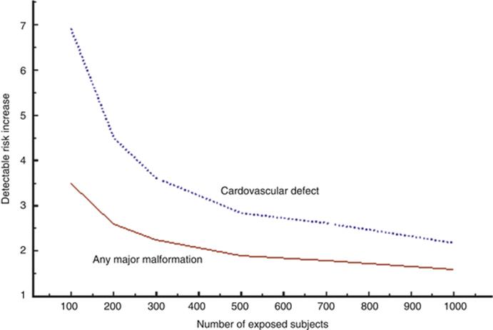
Fig. 9.1
Diagram showing the risk increase detectable at different numbers of exposed subjects for any major congenital malformation (3 % in population) or cardiovascular defects (1 % in population). The exposure rate in the population is supposed to be 2 %
These calculations underline the futility in small studies when they refer to congenital malformations. Only extremely high risks (like that caused by thalidomide) can be detected, and negative studies have very little information value.
9.8 The p-value and Mass Significance
Researchers have a tendency to be blinded by p-values. Here are some common misunderstandings:
· A statistically significant p-value proves that the exposure causes the outcome. First of all it only suggests that the observed association may not be caused by chance – it may be, however, because every 20th time one make a test, the p-value may randomly lie under 0.05 (if that is the significance level, one has determined). These 20 times can be 20 tests made on the same material (looking, for instance, on five different drugs and four different outcomes). This can be corrected for by statistical methods. It could also be one of 20 studies on the same problem, made in different parts of the world, published or unpublished.
Second, the p-value only indicates that there most likely is an association between exposure and outcome, but it may not be causal, the exposure may not have caused the outcome but the association is due to confounding (see above). Sometimes one has to consider the possibility that the outcome has caused the exposure, so-called reversed causality.
· Absence of a statistical significance means that the exposure does not cause the outcome. The correct interpretation is that the study is not large enough (does not have enough power) to show that the observed risk difference is not caused by chance – it may well be true anyway. A p-value of 0.053 or a lower confidence limit of 0.98 is, strictly speaking, expressions of nonsignificance – but common sense should regard such findings as at least suggestive. If the chance for randomness is 1/20 or 1/19 is not that important.
· If one group is statistically significant and, the other is not, the two groups differ. This is no proof that they differ – this has to be shown by an analysis which demonstrates that the risk estimates for the two groups cannot be estimates of the same risk.
Mass significance is an expression of multiple testing that one does not restrict the analysis to one predetermined association but make tests on multiple situations. If we are in the situation that we have a population study where any kind of drug use has been registered and any type of congenital malformation can be studied, we will have the possibility to perform an enormous number of tests – and some of them will come out “statistically significant” just by chance. If we have studied 100 different drugs and 20 different malformations, we can make 2000 tests, and there should randomly be 100 “significant” deviations, either as risks or as protective effects. We will later in this book discuss ways to find out which of them are likely to be true and which are likely random – but it is not possible to do it from the original material.
There are more refined methods of mis-use of mass significance. One way is to start the study mentioned above with 100 drugs and 20 malformations, look for apparent risk increases, and select them for statistical testing, not mentioning the other possible tests which could have been made. The p-value has a meaning only if the test was decided before data were available – one has put this as “a p-value must have a history.” If you decide to make a study of drug A and malformation B and collect data on all drug use and all malformations, you can select the A-B association for testing and the p-value has a meaning. If you did not select the A-B association a priori but did it because it seemed to be interesting, the p-value has no meaning.
Another method to get what you want is to produce a set of different groups and then compare the group with the highest value with the group with the lowest value, again defining such groups from the outcome. If many exposure groups are formed, one has to decide before data are collected which groups to compare.
References
Mantel N, Haenszel W (1963) Statistical aspects of data from retrospective studies of disease. J Natl Cancer Inst 32:719–748
Miettinen OS (1974) Simple interval estimation of risk ratio. Am J Epidemiol 100:515–516