The left ventricular (LV) systolic function is the most commonly ordered and sought after information by a cardiovascular physician because of the diagnostic, therapeutic and prognostic decisions that are made with its help. The LV is a pressurized chamber with a definite architecture. It is a bidirectional asynchronous pump that actively and passively receives blood from the pulmonary circulation and ejects it further into the systemic circulation. Ejection is the part of systole, which has been used to estimate systolic performance most often.
Quantitative and qualitative measures of systolic performance are both determined. The LV contracts and then deforms in systole. However, contraction and
deformation need to be studied separately and together to understand the LV systolic function. Conventional quantitative indexes include the assessment of ejection fraction, ventricular volumes, ventricular mass and wall stress. However, newer and simpler parameters have been explored, which provide useful clinical information and complement the conventional parameters.
MORPHOLOGY OF THE LEFT VENTRICLE
Normal LV comprises of an inlet, apical trabecular, and an outlet portion1 although these portions do not have discrete anatomical borders (Fig. 10.1).
The ventricular wall is thickest near the cardiac base and thins to 1-2 mm at the apex (Fig. 10.2). This is

Fig. 10.1: Three arbitrary parts of the left ventricle. (LVOT: Left ventricular outflow tract).

Fig. 10.2: Myocardial wall thickness and curvature at the apex.
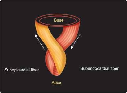
Fig. 10.3: Helical orientation of the myocardial fibers with a figure of 8 near the apex.

Fig. 10.4: Graphic cross-sectional image of the LV. Blue color represents subendocardial descending fibers and the red color depicts outer subepicardial ascending fibers.
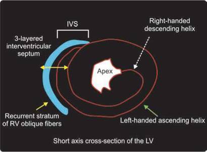
Fig. 10.5: Three-layered structure of the interventicular septum (IVS). The right-sided layer is the inner layer of the right ventricular oblique fibers.

Fig. 10.6: Para-sternal short axis view showing three-layered interventicular septum (IVS) with increased echogenic texture.
responsible for greater wall stress at the apex and more often aneurysm formation.
Transmurally, through the ventricular wall, the myoarchitecture has a typical arrangement of myocardial fibers that change orientation from being oblique in the subepicardium to circumferential in the middle and to longitudinal in the subendocardium (Figs 10.3 and 10.4). ttis helical structure has functional significance.2
Interventricular septum (IVS) is three-layered and hence more echogenic than the rest of the walls. It also thickens less than the rest of myocardium due to its anatomy (Figs 10.5 and 10.6).
the normal LV comprises of an inlet portion containing the mitral valve apparatus, an outlet portion leading to the aortic valve, and an apical portion containing fine trabeculations (Fig. 10.7).
the shape of the left ventricle approximates to a cone or prolate ellipse with the right ventricle hugging it.1 This shape is an evolutionary process to make it most energy efficient (Fig. 10.8).
Fine muscular strands or so-called false tendons that extend between the septum and the papillary muscles or the parietal wall are seen in nearly 50% of all subjects (Fig. 10.9).
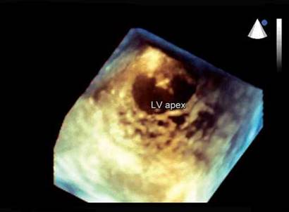
Fig. 10.7: 3D echocardiographic image of the left ventricle (LV) showing fine trabeculations at the apex.
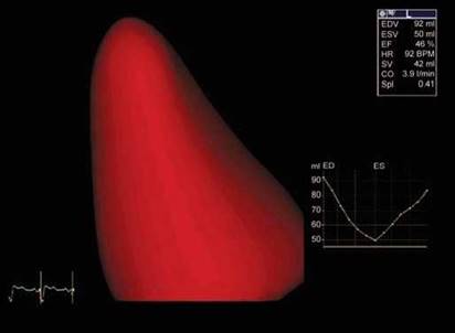
Fig. 10.8: Conical shape of the left ventricle (LV) cavity by 3D echo.
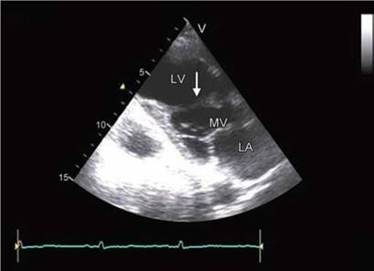
Fig. 10.9: Fibromuscular strand extending between anterior interventricular septum and the posterior wall of the left ventricle (LV).
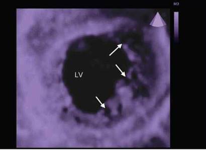
Fig. 10.10: 3D cross-sectional image of the mid-LV. Arrows point to trabeculations and deep recesses.
In many disease states, there are prominent trabe- culations that may make endocardial border delineation difficult. The pathological entity of noncompaction, or spongy myocardium, is characterized by prominent and excessive trabeculations with correspondingly deep recesses in between walls (Fig. 10.10). Herein, automatic endocardial border detection may be a challenge.
The ventricular septum in the normal heart is curved, convexing into the right ventricular cavity. It is muscular except for a small portion immediately beneath the aortic valve, which is a thin fibrous structure, the ventricular component of the membranous septum (Fig. 10.11).
The papillary muscles supporting the mitral valve are an integral component of the left ventricular wall
and participate in the longitudinal function of the LV (Fig. 10.12). These extend from apical third of the ventricular walls to the mitral annulus via tendinous chords.1
Physiology of the Left Ventricle
The LV systole is defined as that part of cardiac cycle wherein active contraction occurs. Typically, it occurs with the closure of the mitral valve and when the LV developed pressure exceeds that of the left atrium.3 Contractile performance is the basis of the LV systolic function. Due to this contraction, when the developed systolic LV pressure exceeds that of aorta, blood is ejected into the latter (Fig. 10.13).
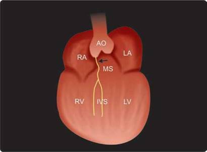
Fig. 10.11: Arrow points to membranous (MS) part of the interventricular septum (IVS).

Fig. 10.12: Graphic apical three-chamber view showing anterolateral (ALPM) and posteromedial (PPM) papillary muscles. The thin chords extending to the mitral valve are the tendinous chords.

Fig. 10.13: Phases of cardiac cycle of the LV.
(IVCT: Isovolumic contraction time; ITC: Isotonic contraction, ITR: Isotonic relaxation).

Fig. 10.14: The left ventricular pressure-volume loop. Width of the loop represents stroke volume (SV) and area of the loop is stroke work. (IVC: Isovolumic contraction; (IVR: Isovolumic relaxation).
The total blood ejected into aorta in one cardiac cycle is stroke volume (SV) and the work done to achieve this SV is called stroke work. At the end of systole, the volume left in the LV (end-systolic volume) and the end-systolic pressure are indicative of intrinsic LV contractility, and the SV and stroke work represent systolic function and more accurately when normalized for the end-diastolic volume.4 ttese functions can be accurately depicted by the LV pressure-volume loop (Fig. 10.14).
Pressure-volume loop cannot be studied nonin- vasively. However echocardiography helps to estimate SV, end-systolic volume and ejection fraction (SV/end-
diastolic volume), the commonly used parameters of the LV systolic function.
the LV systole has two parts:
1. Isovolumic contraction (IVC)
2. Ejection
Ejection is further divided into rapid ejection (isotonic contraction) and slow ejection (isotonic relaxation)
the LV function can be studied in all these four phases of tension-time sequence (Fig. 10.15). Combined myocardial performance index is a ratio of isovolumic time/isotonic time and provides information about systolic and diastolic function. This can be obtained by

Fig. 10.15: The left ventricular tension-time sequence.

Fig. 10.16: Myocardial tissue velocity spectrum in a single cardiac cycle. Rate of tissue motion or deformation (systolic velocity) peaks in early systole coinciding with peak of isotonic contraction.
Fig. 10.17: Common indices of systolic function like fractional shortening, ejection fraction and mitral annular systolic excursion are measured at end-systole.

Fig. 10.18: Graphic depiction of the LV showing three major vectors of deformation.
(L: Longitudinal; R: Radial and circumferential).
Doppler echocardiography.5 Rate of maximum pressure development (dP/dT) is measured during IVC phase and is afterload independent. This can be obtained from the continuous wave (CW) Doppler signal of mitral regurgitation.6
Tension development peaks in early systole while the maximal deformation of the LV occurs at end-systole or slightly beyond it (Figs 10.16 and 10.17). Hence, there are two types of LV systolic function indices commonly studied7:
1. Peak systolic indices
2. End-systolic Indices
Peak systolic velocity indices [mitral annulus tissue velocities, ejection velocities, and strain rate (SR)] exhibit
greater variation than end-systolic indices during inotropic alterations from which it is assumed that they better reflect LV contraction (Figs 10. 16 and 10.17).
End-systolic indices are less sensitive to heart rate manipulation compared to peak systolic indices. However, it is not clear if there are significant differences between the two types of indices.
Development of tension results in deformation. Systolic function is a manifestation of deformation. There are four recognizable vectors of deformation (Fig. 10.18)
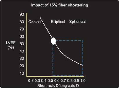
Fig. 10.19: Relationship of left ventricle ejection fraction (LVEF) with shape of the left ventricle for a fixed 15% long-axis shortening.

Fig. 10.20: Determinants of left ventricle systolic function.

Fig. 10.21: Relationship of velocity of shortening and afterload. With increasing preload, the curve shifts upward.
1. Longitudinal shortening
2. Radial thickening
3. Circumferential shortening
4. Rotation
Complex interplay of these vectors of deformation results in energy-efficient systolic function. These deformation indices also provide useful information about the systolic function. Longitudinal deformation indexes are getting accepted for clinical use although other types of deformation are under active validation.8
There is a relationship between longitudinal deformation and the left ventricular shape. Longitudinal shortening is a good surrogate for global systolic function (Fig. 10.19).
Determinants of LV Systolic Function
For a certain degree ofcontractility (the intrinsic contractile strength of the myocardium), the SV of the ventricle, which is the most obvious systolic function parameter, is determined by the preload (the end diastolic ventricular volume, pressure or stretch), afterload (the force opposing ejection) and the heart rate, which has biphasic effect of increasing contractility and reducing diastolic filling period (Fig. 10.20).
Contractility can be altered by adrenergic stimulation, heart rate and calcium.
To some extent, preload-adjusted parameters can be estimated by using end-diastolic length or volume as the denominator, the most prominent example of which is ejection fraction wherein SV is indexed for end-diastolic volume.
Physiological Principles Governing LV Systolic Function3
• Starling's law: Ability of the heart to change its force of contraction and therefore SV in response to changes in venous return is called the Frank-Starling mechanism (or Starling's Law ofthe heart). Increasing the sarcomere length increases troponin C calcium sensitivity, which increases the rate of cross-bridge attachment and detachment, and the amount of tension developed by the muscle fiber (Figs 10.21 and 10.22)
• Bowditch effect: It is an autoregulation method by which myocardial contractility increases with an

Fig. 10.22: Relationship between the preload [end-diastolic volume or end-diastolic pressure (EDV and EDP)] and the SV.

Fig. 10.23: Relationship between force developed and the heart rate.

Fig. 10.24: The method of measuring wall stress.
increase in heart rate. Also known as the Treppe phenomenon, Treppe effect or staircase effect (Fig. 10.23). Mechanism is that the Na+-Ca+ membrane exchanger, which operates continually, has less time to remove the Ca++ that arrives in the cell because of the decreased length of diastole with positive chronotropy. With an increased intracellular Ca++ concentration, there follows a positive inotropy.3
• Laplace's law: the Laplace's law governs the relationship of wall stress to radius and wall thickness in presence of a given amount of force generated by the LV. Wall thickening increases to maintain normal wall stress whenever the LV dilates. Increased wall stress is the initial manifestation of the declining systolic function (Fig. 10.24). End-systolic volume normalized
for end-systolic wall stress is a fairly good index of systolic elastance or contractility.
Base of the heart, referred to as the atrioventricular (AV) plane or ring, moves toward the apex during systole, and the apex makes very slight movements.9 Long axis motion of the mitral annulus reflects the function of longitudinally oriented left ventricular myocardial fibers (Fig. 10.25) ttis rapid motion of the mitral annulus is dependent on stored energy from the previous systole and contributes significantly to LV (suction and early) filling in normal hearts.
the normal mean mitral annular total amplitude of motion in healthy adults ranges from 10 mm to 15 mm. ttese values may be higher in younger subjects and have been reported to decline from 15 mm at 20-40years to about 10 mm at 61-80 years.10
Characteristically, when the overall long-axis amplitude is low, peak shortening and lengthening rates are reduced and global ejection fraction is reduced.11 Methods to study long axis function are:
• Mitral annulus plane peak systolic excursion (MAPSE) by two-dimensional (2D)-directed M-mode (Fig. 10.26)
• Tissue tracking or displacement by color Doppler myocardial imaging
• Peak systolic velocity of the mitral annulus by tissue Doppler imaging
• Use of 2D or three-dimensional echocardiographic (3DE) methods to study long-axis shortening from

Fig. 10.25: Graphic depiction of descent of the LV base during systole and longitudinal expansion during diastole.
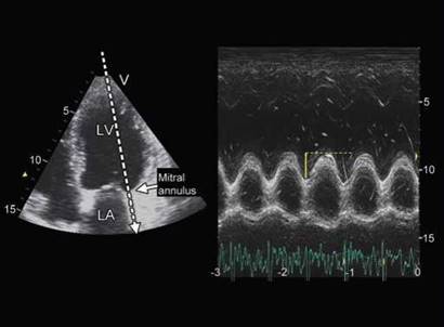
Fig. 10.26: Mitral annulus plane systolic excursion (MAPSE) by 2D-guided M-mode from apical view.
apical endocardial peak to midpoint of mitral annulus in apical views.
• The 2D-targeted M-mode beam is directed from the apex along the hinge points of the mitral valve apparatus and lateral, septal, inferior, anterior and posterior LV walls in four-, two- and three-chamber views.
• The regional displacement is calculated after 60 ms from the beginning of the QRS complex to the first peak of the mitral annular waveform.
• To normalize MAPSE measurements, the longitudinal LV inner distance is measured from the apical endocardial border to the AV plane at the end of diastole.
• Anatomical M-mode is used to overcome limitations with regards to parallel alignment of the M-mode beam to the plane of mitral annulus.
• Color tissue Doppler M-mode can be used as an additional method to assess the amplitude of MAPSE, as this technique ensures high spatial and temporal resolutions.
• Tissue tracking algorithm of the color Doppler myocardial imaging can provide this information off-line.
A comprehensive quantitative assessment of end-systolic
and end-diastolic volumes of the entire left ventricle is
most sought after information to obtain ejection fraction
and to monitor the LV remodeling. It is best provided by the 3DE with semiautomated or automated edge- detection algorithms. However, in clinical practice, 1 or 2D echocardiographic techniques are commonly used with geometric assumptions to obtain LV volumes. Typical simplifications, which require only a limited number of measurements, are currently made based upon geometric assumptions of the left ventricular geometry.12 All assumptions more closely approximate 'true' left ventricular chamber sizes when the heart is normal, resulting in greater errors when there is global enlargement or dysfunction. The greatest errors occur in settings of regional anatomic distortion or systolic dysfunction. A summary of these is given below:
Cube Formula and its Modification
M-mode calculations of LV volumes assume that the LV is a prolate ellipse and that by measuring a single minor axis dimension and cubing it, volume can be calculated.
The volume of a cube is based upon a single left ventricular measurement of midcavity diameter (LVID), which is derived from M-mode data obtained from the 2D para-sternal long- or short-axis view. Volume is derived from the following formula:
Volume [V] = D3
Teichholz modified this formula for better correlation with other methods of volume estimation.13
The Teichholz equation
Volume = [7/(2.4 + LVID)] x [LVID]3
Although commonly present in most echocardio- graphic calculation packages, it has been given up due to inaccuracies (Fig. 10.27).

Fig. 10.27: Minor axis diameter obtained can cause marked variations in volume calculation by cube formula.

Fig. 10.28: Single-plane ellipsoid formula to estimate volume.

Fig. 10.29: Biplane ellipsoid formula to estimate LV end-diastolic volume. There is a difference of 10 mL volume between the two planes.
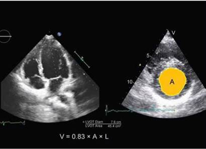
Fig. 10.30: Bullet method to estimate left ventricle volume. (LVOT: Left ventricle outflow time).
Single-Plane Ellipsoid
the volume of a single-plane ellipsoid uses left ventricular length (L) and midcavitary area (A) measurements obtained from the apical four-chamber view (Fig. 10.28). the volume may be calculated as follows:
Volume = 0.85 x A2/L
Biplane Ellipsoid Formula (Biplane Area-length Method)
The volume formula using a biplane ellipsoid employs left ventricular length (L) and area (A) measurements obtained from the apical four-chamber view (A1) as well as two-chamber view (A2). the smaller of the two lengths is used as denominator (Fig. 10.29).
Volume = 0.85 x A1 x A2/L t
min
Bullet Formula
The volume of a bullet shape uses the left ventricular length (L) from the apical four-chamber view with the left ventricular chamber area (A) from the para-sternal short- axis midcavity view (Fig. 10.30).
Volume = 0.83 x A x L
Modified Simpson's Rule (Disk Summation Method)
The modified Simpson's rule determining left ventricular volume consists of a summation of discs using a measurement of the left ventricular length (L) from the apical four- chamber view and the two-chamber view. Height of each disc is predetermined and discs are placed equidistant

Fig. 10.31: Modified Biplane Simpson or disk summation method to estimate LV volumes. Disks are stacked from base to apex at equal distance.

Fig. 10.32: Modified Quinones Method. Measurement of midcavity diameters and qualitative assessment of the apex.
(LVEDD: Left ventricular end-diastolic diameter; LVESD: Left ventricular end-systolic diameter).
(Fig. 10.31). Biplane method of discs is recommended by the American Society of Echocardiography.12
The modified Quinones method is commonly used and employs linear measurements.14 It uses single measurements of the LV cavity in the midventricle in both end-diastole and end-systole, and can be employed using either M-mode or 2D imaging (Fig. 10.32).
• Because only two linear measurements are needed, the modified Quinones method often requires less time to perform than other methods and only needs adequate visualization of the endocardium in the midventricle.
• However, because this method only measures circumferential contraction in a single plane, significant assumptions about LV chamber geometry have to be made so that a change in a linear measurement can act as a surrogate for a change in volume.
• the contribution from longitudinal contraction on LVEF is not directly measured, but rather a correction factor is used to adjust the measured LVEF based on a visual grading of the apical contraction.
• In situations where there is asymmetry of contraction, such as in ischemic LV dysfunction, this method has significant limitations.
With the modified Quinones method, the cavity size can be overestimated if the ultrasound beam/image is not perpendicular to the ventricular cavity, or underestimated if the ultrasound beam/image is not in the center of the cavity.

Endocardial Border Delineation
For LV volumetry, accurate endocardial border delineation is paramount. This can be performed using:
• Harmonic imaging.
• Use of contrast for chamber opacification (Fig. 10.33).
• Automatic endocardial border detection.
• Left ventricular ejection fraction (LVEF) is the fraction of blood pumped out of the LV with each heart beat. It can be measured by the invasive methods and noninvasive methods like gated blood pool heart scan, computerized tomography, cardiac magnetic resonance imaging and echocardiography.
• In a clinical situation, LV volumes and EF measurements for a specific patient are classified as normal or abnormal based on established normal limits. Although LV ejection fraction is a continuous biological variable, a value < 55% has been termed abnormal by the recent guidelines of the American Society of Echocardiography (ASE).

Fig. 10.33: Apical four-chamber (left) and two-chamber (right) views with chamber opacification with Sonovue. Contrast use makes endocardial border stand out. But plane of mitral annulus may be difficult to identify.

Fig. 10.34: M-mode measurements can be obtained using 2D echo- cardiographic guidance from parasternal long-axis or short-axis views.
• Prognosis and therapeutic decisions are often based on left ventricular ejection fraction (LVEF), which means the LVEF needs to be accurately measured.
• Reference values for normal people:12
LV end-diastolic volume index 35-75 mL/m2 LV end-systolic volume index 12-30 mL/M2
LVEF >55%.
• A temporal variability in ejection fraction (EF) of 5% might occur with 3DE due to physiological differences and measurement variability, whereas this might be >10% with 2D methods. Overall, 3DE has the best intra- and interobserver as well as test-retest variability.15
M-mode echocardiography has fallen in disrepute as a technique to assess LV systolic function because of significant limitations. However, some people still continue to use it under 2D-echocardiographic guidance. It is the simplest way to obtain LV dimensions and wall thickness and if obtained with anatomical M-mode (a technique to steer the cursor so that it remains perpendicular to the LV walls), is reasonably accurate.16
Left ventricular chamber size reduction during systole is the consequence of the simultaneous contraction of myocardial layers in the different directions, yielding the three basic left ventricular geometric changes: reduction of minor axis, shortening of long axis and twisting of the
apex. M-mode echocardiography can be used to estimate the first two changes.
However, minor axis shortening is a valid surrogate of global systolic function only if the ventricle contracts symmetrically and without any geometric alteration (Fig. 10.34).
M-mode echocardiography has been used to estimate:
• LV dimensions.
• LV wall thickness.
• Fractional shortening of the LV.
• Circumferential fiber shortening.
• Velocity of circumferential fiber shortening.
• Ejection fraction by modified cube formula.
• Midwall shortening fraction.
• Meridional wall stress (using LaPlace law).
• Mitral E point-Septal separation distance.
• Relative wall thickness.
• Segmental wall motion abnormality confined to anterior interventricular septum (IVS) or posterior wall. Endocardial fractional shortening is usually preserved
while midwall fiber shortening is reduced with onset of systolic dysfunction. In fact, there is an epicardium-to- endocardium thickening gradient in systole, which is a better index of systolic function than one-dimensional endocardial shortening alone.
The magnitude of systolic shortening measured at the endocardium does not directly reflect the intramural shortening.

Fig. 10.35: M-mode cross-sectional view at the level of mitral leaflets with various measurements shown on the right side of the image.

Fig. 10.36: Measurement of LV ejection time (ET) from the box-like opening of the aortic valve.

Fig. 10.37: M-mode of the basal part of the LV showing mitral E point very close to IVS indicating normal systolic function.

Fig. 10.38: Increased EPSS in a patient with LV systolic dysfunction.
• M-mode tracing is obtained by placing the cursor just beyond the tips of the mitral valve leaflets in 2D-echocardiographic para-sternal long-axis view (Fig. 10.35).
• Ultrasound beam is kept parallel to the IVS.
• Measurements are made by leading-edge method, using R wave on ECG as the end-diastole and the peak of LV posterior wall thickening as the end-systole. (Fig. 10.35).
• LV dimensions and wall thickness are measured both at end-diastole and end-systole.
• Ejection time (ET) is measured from the M-mode tracing of the aortic valve (Fig. 10.36).
• Mitral valve E points to IVS distance (EPSS) in early diastole is measured as an indirect index of LV systolic dysfunction (Figs 10.37 and 10.38).
Measurements: Following measurements and calculations are made:
• LV end-diastolic dimension (normal 3.5-5.3 cm).
• LV end-systolic dimension (2.5-3.9 cm).
• LV fractional shortening (LV diastolic dimension minus end-systolic dimension divided by end-diastolic dimension x 100, normal values 27-45%).

Fig. 10.39: Estimation of velocity of circumferential fiber shortening. Ejection time is obtained from the aortic valve (right panel).

Fig. 10.40: M-mode image of the mitral valve (above) and aortic valve (below) and M-mode of the color tissue velocity image of the posterior wall. Note prolonged isovolumic contraction period (before aortic valve opening) and also isovolumic relaxation period (aortic valve mitral valve opening). There is continued thickening of the posterior wall during IVRT indicative of systolic dysfunction.
(AVO: Aortic valve opening; MVO: Mitral valve opening; AVC: Aortic valve closure).
• LV ejection fraction, which is automatically calculated by the system using Teichholz method.
• Velocity of circumferential fiber shortening (Normal > 1.0 circumference/s) (Fig. 10.39).
• the 2D-guided mitral plane systolic excursion (MAPSE). An average value of medial and lateral edge is normally > 12 mm and corresponds well to 3D ejection fraction.
• Measurement of circumferential left ventricular shortening in the middle of the diastolic wall thickness (midwall shortening17).
Limitations of M-mode Echocardiography16
• Limited ice pick view of the LV (accuracy will depend upon the slice being examined).
• Measurements not valid for asymmetric ventricles.
• Errors due to nonparallel cursor.
• Geometric assumption in measurement of ejection fraction.
• Paradoxical motion of IVS (LBBB, postoperative, RV volume overload) leads to false and inaccurate functional parameters.
current use of M-mode Echocardiography in LV systolic Function Assessment
• Measurement of MAPSE
• Myocardial performance index can be measured by sweeping the beam from mitral valve to aortic valve to get opening and closing of both valve leaflets in a single image
• M-mode color flow propagation velocity of the mitral valve to get early diastolic suction effect and hence indirect idea about systolic function
• M-mode of the tissue color Doppler images to understand physiology better with high temporal resolution (Fig. 10.40)
2d Echocardiography and LV Systolic Function
2D Echocardiographic Minor Axis Shortening
Minor axis endocardial shortening has been considered a valid surrogate for regional ejection fraction (Fig. 10.41) and could also be used for global function in case the LV is contracting symmetrically and a constant is used for apical myocardial behavior.
However, endocardial shortening becomes a poor indicator of LV function in presence of increased wall thickness, concentric remodeling and in presence of segmental asynchrony.
• Systolic shortening of longitudinally oriented subepicardial and subendocardial fibers squeezes the circumferentially oriented fibers at the midwall level, thereby potentiating cross-fiber myocyte thickening and cross-fiber left ventricular radius shortening.
• Ventricular radius shortening at the endocardium is the consequence of the interaction of contraction and thickening of differently aligned myocardial muscular layers located at a distance.

Fig. 10.41: Endocardial shortening fraction at the level of chordae tendinae. Normal values are 27-45%.

Fig. 10.42: 2D echocardiographic parasternal long axis view showing method of assessing circumferential fiber shortening.

Fig. 10.43: Midwall fiber shortening, a technique that was in great vogue before the advent of acoustic speckle tracking for cross-fiber function.
• Endocardial radius shortening provides much less information about systolic function compared to midwall shortening or circumferential shortening (Figs 10.42 and 10.43).
2D Echocardiographic Ejection Fraction
Although eyeballing for estimation of ejection fraction from 2D echocardiographic views is quite in vogue,18 most laboratories still measure LV volumes. The most commonly used and recommended method is biplane Simpson method because it has least geometric assumptions.19 It is also possible to create an automatic grid by marking two points of the mitral annulus and the apex. The grid can then be manually modified to correctly trace endocardium.
Technical Tips for LV Volume Estimation by the Simpson Method
• End-diastole and end-systole are identified from 2DE cine-loops using frame-by-frame analysis of the apical four- and two-chamber LV views as the largest and smallest cavity during the cardiac cycle, respectively.
• Tracing of endocardial border is manually done in both frames, paying attention to include the papillary muscles within the LV cavity.
• Left ventricular ejection fraction is automatically calculated by the software using the biplane disk- summation algorithm (modified Simpson's rule).
• Use of biplane imaging makes it easier to estimate volumes of the two views in the same frame. It also allows alignment of the cursor to define apex better.
• Border detection can be improved by use of harmonic imaging and with optimum sector width.
• Volume-time curves can also be generated using vendor's software.
• Fully automated measurements with no manual correction of LV volumes produce an underestimation of LV volumes in comparison with manually corrected ones.
• High image quality is a prerequisite for any border- detection method and no less dependent on the operator's expertise in image acquisition. All efforts should be made to obtain crisp endocardial delineation in as many segments as possible.
• If there are more than two segments showing endocardial dropouts in any view, contrast should be liberally used for chamber opacification20 (Fig. 10.44).
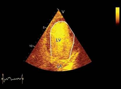
Fig. 10.44: LV opacification by a contrast agent. It is easy to include papillary muscles and trabecular recesses in the cavity by this technique to get larger volumes than by standard 2D gray-scale imaging. Note quantitative analysis of the LV volumes by 2D echocardiography is highly experience-dependent and uses only partial information about cardiac anatomy and function contained in predefined cross-sectional views. Therefore, it may be subject to substantial measurement errors, particularly in patients with regional wall-motion abnormalities and/or distorted LV geometry.21
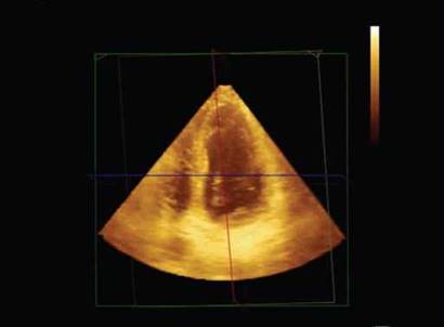
Fig. 10.45: Full-volume data set recorded from an apical view.
Limitations of 2D Echocardiography for LV Volume Estimation
• Geometric assumptions for estimating volume, which may not be valid.
• Apical foreshortening (typically, long-axis diameter in an adult should be > 8 cm: failure to achieve this, indicates apical foreshortening).
• Off-axis imaging (plane positioning error).
• Translation and rotation from diastole to systole.
• Suboptimal images and difficulties in tracing the entire endocardium.
• Challenge of endocardial delineation in situations of hyper-trabeculation.
• High intraobserver, interobserver and test-retest variability.
• Operator-dependent and requires experience.
Real-time 3d Echocardiography for Study of LV Systolic Function
Real-time 3D-echocardiography obviates the limitations inherent in 2D echocardiographic volumes and ejection fraction estimation.21,22 It is possible to obtain these measurements within minutes using various algorithms
built in the systems. The key to 3D imaging is a matrix-
array transducer and an inbuilt software algorithm for 3D
calculation.
Method of 3D Volumetry and Ejection Fraction Measurement
• In a system capable of 3D imaging, a full-volume data set is recorded in held respiration, using a matrix array transducer in any apical view over 4-6 beats (Fig. 10.45). In this way, a pyramidal 3D data set of 90° x 90° is obtained at a frame rate of 20-25 Hz.
• the pyramidal volume data set is transferred to 3D calculation package. The volume data set is usually recorded in 4-6 beats and these volume slices are stitched together to get a pyramidal set. It is also possible to obtain full volume data set in one cardiac cycle although temporal resolution is usually suboptimal (Fig. 10.46).
• In multiplane reconstruction mode, the system displays two or more apical images, one or none short-axis image and one pyramidal data set in a quad screen format (Fig. 10.47).
• Using longitudinal and horizontal cursors, longest apical views with best endocardial delineation are obtained.
• The software guides to place points on the two edges of the mitral annulus and at the peak of endocardium at the true apex both in end-systole and end-diastole.
• the endocardium is traced > 700 points. Manual correction is frequently performed for optimization of endocardial tracking.

Fig. 10.46: Pyramidal full volume data set acquired in 4 cardiac cycles.

Fig. 10.47: Multiplane reconstruction of the 3D full volume data set.

Fig. 10.48: 3D reconstruction of the LV cavity from the tracked endocardium. Graph below shows regional volumes with marked end-systolic volumes.
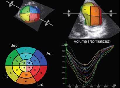
Fig. 10.49: Display of 3D data set calculation. All 16-segments contract to reach end-systolic volume nearly simultaneously in this subject.
• Once endocardial delineation and tracking is accepted by the operator, the system automatically calculates regional and global volumes and ejection fraction along with systolic dyssynchrony index (Figs 10.48 and 10.49). The software creates a mathematical model or 'cast' of the LV, which allows time- volume calculations to be performed for the entire cardiac cycle.
• If there are stitch artifacts, the data set needs to be discarded.
• Further parametric calculations for onset of contraction and amount of shortening in various regions can also be displayed in bull's eye map.
In a ventricle with synchronous contraction of all segments, one expects each segment to achieve its minimum volume at almost the same point in the cardiac
cycle, whereas in a dyssynchronous ventricle there will be a dispersion in the timing of the point of minimum volume for each of the 16 or 17 segments. The degree of dispersion can be calculated by measuring the standard deviation of the time to achieve minimum volume and then correcting that for the R wave to R wave (R-R) interval. This allows derivation of a systolic dyssynchrony index, which can be used to quantify the degree of LV dyssynchrony from a comparison of all segments (Fig. 10.50).
Advantages of 3D Echo
• Low intraobserver and interobserver variability.
• Automatic endocardial delineation with small manual correction; 3D measures endocardial position at > 700 points.
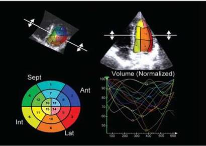
Fig. 10.50: Marked dyssynchrony shown by greater dispersion of regional end-systolic points.

Fig. 10.51: 3D volumes, ejection fraction and systolic dyssynchrony index ( SDI) displayed simultaneously. An SDI of < 8% is considered normal.

Fig. 10.52: Annular tissue velocities recorded from the lateral edge of the mitral annulus. Arrows point to peak systolic velocity. First systolic wave during ejection is due to contraction of longitudinal fibers.
• High concordance with 'gold standards' like cardiac magnet resonance imaging.
• No geometric assumptions.
• Regional volumes and functions can be studied with ease.
• Better description of sphericity index (calculated by dividing the LV end diastolic volume (calculated from a 3D data set) by the volume of a sphere, the diameter of which is the LV major end diastolic long axis).
• Analysis of regional function in time domain and study of intraventricular dyssynchrony.
• Patients with a higher dyssynchrony index have a lower ejection fraction (Fig. 10.51).
• Parametric 'bulls eye' displays of the timing of LV contraction are also available.
• The details of how the endocardium is traced are important.
• Spatial resolution of 3D echocardiography is still limited.
• the trabeculae may be attributed to the LV wall.
• the reliability of automated correction methods that can be used to track the compacted myocardium seems encouraging but warrants further study.
• the application of contrast during 3D imaging may improve some of these problems but continues to pose challenges that relate to the definition of the mitral annular plane.
• the optimal balance between multibeat imaging, which offers better spatial resolution but has the risk of stitching artifact, and single-beat acquisitions remain to be elucidated.
• Studies have demonstrated differences between online and offline measurement of LV volumes, possibly related to differences in the automated detection algorithms.
• Intervendor differences need to be sorted out.
All in all, 3DE estimation of ejection fraction and dysynchrony index is likely to replace 2D parameters in near future.
Systolic Velocities of the Mitral Annulus
During the ventricular ejection period, longitudinal shortening of the LV can affect the movement of mitral annulus and produce S' wave (Fig. 10.52), which is peak annular systolic velocity.23

Fig. 10.53: Marked difference in S' velocity on medial versus lateral edge due to wall motion abnormality.

Fig. 10.54: A peak's velocity of 5 cm/s (medial edge of the mitral annulus) in a subject with dilated cardiomyopathy and ejection fraction of 30%.
The systolic motion of the mitral annulus is not entirely due to myocardial longitudinal shortening or contraction but rather is the summation of contraction and rotation. Apical rotation itself can be regarded as a main driving force of longitudinal shortening
These velocities are measured with ease, less influenced by the loading condition of the LV and have low inter- and intraobserver variability.
Tips to Record Mitral Annular Velocities
• Mitral annular longitudinal velocities are recorded using pulsed-wave mode by positioning the Doppler cursor with a 5 mm sample volume at the lateral, septal, inferior, anterior and posterior AV margins in LV tissue Doppler apical images.
• Care is taken to ensure that the ultrasound beam is kept parallel to the mitral annular motion.
• The filters and gains are set low in accordance with the recommendations for quantification of Doppler echocardiography.
• Peak systolic velocity is measured avoiding the initial peak that is observed during IVC time. However, during ejection also, there can be two peaks, usually at the lateral edge. The first systolic wave represents contraction of longitudinal fibers.
• The advantage of mitral annular velocities is that these are not dependent upon quality of images.
A good association between S' and apical rotation under a variety of LV inotropic conditions has been shown.
• The location of tissue Doppler sample volume is another issue in the assessment of global LV contractility. The major advantage of the medial (septal) mitral annulus is that the ultrasound beam is most parallel to the LV longitudinal movement.24
Global left ventricular function can be estimated by recording mitral annular systolic velocity. The implementation of a cutoff limit of 8 cm/s gives a simple guide for differentiating between normal and abnormal left ventricular systolic function that might be useful clinically in patients without regional wall-motion abnormalities. However, in patients with important segmental wall-motion abnormalities during systole, left ventricular longitudinal shortening may be an imperfect surrogate for ejection fraction (Fig. 10.53).
The best differentiation of normal (> or = 50%) from abnormal (< 50%) ejection fraction is provided by peak systolic velocity > or = 8 cm/s for the medial (sensitivity 80%, specificity 89%) or lateral (sensitivity 80%, specificity 92%) mitral annulus.25
Vinereanu et al.25 showed that 90% of the patients with systolic heart failure (LVEF < 50%) had impaired mitral annular systolic velocity less than 7.05 cm/s. Park et al.26 compared their data of mitral annular systolic velocity (medial edge) of less than 6.8 cm/s with 3DE ejection fraction, which showed best sensitivity, specificity of 94% and 87%, respectively, for systolic dysfunction (LVEF < 50%) (Figs 10.54 and 10.55).
A rest-stress difference of > 2.0 cm/s in S' velocity indicates myocardial reserve that can be of help in detecting myocardial viability.27
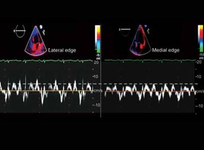
Fig. 10.55: Same patient as in Fig. 10.54. Note about 1cm/s S' velocity difference between two sites.

Fig. 10.56: Graphic display of estimation of the LV dP/dt from CW mitral regurgitation signal.

Fig. 10.57: dP/dt of 572 mm Hg/sec in a patient with dilated cardiomyopathy and ejection fraction of 28%.
the dP/dt of the LV as a Doppler Measure of contractility
the LV contractility dP/dt can be estimated by using time interval between 1- and 3m/s on MR velocity CW spectrum during isovolumetric contraction, that is, before aortic valve opens when there is no significant change in LA pressure (Figs 10.56 and 10.57).28
32
dP/dt=
T
Left Ventricular outflow tract Velocity time Integral
Left ventricular outflow tract velocity-time integral (LVOTvti) is an effective and noninvasive method when
assessing LV systolic function under conditions of varying preload, heart rate, and inotropic state (Fig. 10.58)
LVOTvti is thought to be a better indicator of LV systolic function than is SV, without the confounding factor of LVOT-area measurements.
the Doppler VTI method in estimating SV and cardiac output correlates well with results of concurrent thermodilution cardiac output determinations in patients without significant left-sided valvular regurgitation.
Normal values range from 17 cm to 24 cm. Its best use lies in emergency care where serial measurements may be important to assess SV.
ttis is also the parameter most often used for optimizing resynchronization therapy.29
Global Longitudinal Strain and Strain Rate
With tissue Doppler imaging and speckle tracking, quantification of the LV function has moved beyond the simple ejection fraction measurements and wall-motion score.
Systolic dysfunction might be initially apparent in the longitudinal direction because subendocardial fibers, which are the ones more vulnerable to myocardial ischemia and fibrosis, are longitudinally oriented (Fig. 10.59).
Systolic longitudinal strain is defined as the percent shortening of the myocardium during the systole and its rate of shortening is called SR. Typically, global longitudinal strain of the LV exceeds -15% and SR exceeds 1/s-1.
Strain parameters can be estimated using tissue Doppler technique (unidimensional) or acoustic speckle

Fig. 10.58: Estimation of LVOTvti in a normal subject.
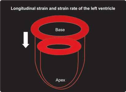
Fig. 10.59: Graphic description of longitudinal shortening of the LV during systole.

Fig. 10.60: Longitudinal strain (left panel) and strain rate (right panel) by myocardial Doppler technique. Peak longitudinal strain of basal interventricular septum (IVS) is -12% and peak strain rate is 0.8 s-1.
tracking (2D or 3D). Tissue Doppler-based strain is slightly higher due to greater temporal resolution (Figs 10.60 and 10.61).
Non-Doppler 2D strain by acoustic speckle tracking is angle-independent, easy to use and provides both regional and global strain from gray-scale images. It has lower temporal resolution than the Doppler-based method but is more reproducible (Fig. 10.62).
Strain and SR measurements are well documented and validated tools for the quantification of myocardial
function.30 While strain correlates with SV and ejection fraction, SR has strong correlation with dP/dt. The potential for detecting subclinical LV systolic dysfunction by the alteration of longitudinal strain is the premise for its use in clinical conditions.31
trough longitudinal strain analyses in four-chamber, two-chamber and apical long-axis views, both regional (relative to each of the 16 or 17 LV segments) and global strain values (global longitudinal strain) can be obtained (Fig. 10.63).

Fig. 10.61: Acoustic speckle tracking of the IVS showing spectrum of longitudinal strain in right upper panel (-11%).
Global longitudinal strain is a superior outcome predictor compared to the EF and wall-motion score index.32 Further, significant correlation between global LS and e confirms the link between systole and diastole.
Method of Assessing Longitudinal Strain
• Using commercially available 2D strain software, the endocardial border in the end-systolic frame is manually traced.
• Three apical views are used to estimate global LS.
• A region of interest is drawn to include the entire myocardium. The software algorithm automatically segments the LV into six equidistant segments and selects suitable speckles in the myocardium for tracking.
• The software algorithm then tracks the speckle patterns on a frame-by-frame basis using the sum of absolute difference algorithm.
• Finally, the software automatically generates time- domain LV strain profiles for each of the six segments of each view from which end-systolic strain was measured (Fig. 10.60).
• The average value of strain at each level (basal, middle and apical) and global strain obtained from averaging the strain values of 16 or 17 LV segments is calculated (Fig. 10.63).
Advantages of Longitudinal strain and Strain Rate Analysis
• Good correlation between longitudinal strain and the left ventricular ejection fraction.
• Longitudinal strain provides a quantitative myocardial deformation analysis of each LV segment, also allowing for early systolic dysfunction detection in patients with a preserved LVEF.
• Sub clinical systolic dysfunction assessment when ejection fraction and other parameters are normal.
• Incremental prognostic value in a variety of diseases like heart failure, postmyocardial infarction, valvular heart disease, and so forth.
• Limits of agreement between various speckle-tracking software are narrower for global longitudinal strain, making it a more robust parameter than the radial or circumferential strain.

Fig. 10.62: Unifrom 2D longitudinal strain extracted from all the six segments in the four-chamber view in a normal person. Average longitudinal strain is -22% and there is very little temporal dispersion.
limitations
• Strain analysis is contingent on the presence of adequate echocardiographic views.
• It is not possible to conduct strain measurements in patients with nonsinus rhythms.
• Results depend critically on the machine with which the analyses are performed, and these are not interchangeable among different manufacturers at least as of now.
summary
There are many ways in which LV function can be
determined, but every measure that is commonly used
is only a surrogate marker of LV function due to the fact that it is impossible to characterize the complex geometric and volumetric function of the ventricle in a single number. ttere is no one perfect measure of LV function. The ejection fraction has emerged as the pre-eminent method to express LV performance. Although ejection fraction is universally accepted, there are a number of other techniques that can assess LV function and, when taken together, provide a more comprehensive picture both of global and regional LV function. Each of these measures (including ejection fraction) has variable dependence on loading conditions, heart rate and geometric position that limits its accuracy. Understanding the limitations of each measure will allow the physician to more intelligently understand the true status of the myocardium.

Fig. 10.63: Global longitudinal strain from three apical views in a patient with aortic stenosis. Global longitudinal strain is -10.5% and shows marked heterogeneity.
In short, LV systolic function should be assessed by a multiparametric approach that includes LV geometry, ejection fraction, long axis function, global longitudinal strain and time-domain function like ratio of isovolumic to ejection periods and so forth.
references
1. Ho SY. Anatomy and myoarchitecture of the left ventricular wall in normal and in disease. Eur J Echocardiogr. 2009;10: iii3-iii7.
2. Greenbaum RA, Ho SY, Gibson DG, et al. Left ventricular fibre architecture in man. Br. Heart J. 1981;45:248-63.
3. Guyton AC, Hall JE. Textbook of medical physiology, 11th ed. Philadelphia, PA: Elsevier Saunders; 2006.
4. Sagawa K. the end-systolic pressure-volume relation of the left ventricle. Definition, modifications and clinical use. Circulation. 1981;63:1223-27.
5. Tei C. New non-invasive index for combined systolic and diastolic ventricular function. J Cardiol. 1995;26:135-6.
6. Bargiggia GS, Bertucci C, Recusani F, et al. A new method for estimating left ventricular dP/dt by continuous-wave Doppler echocardiography. Validation studies at cardiac catheterisation. Circulation. 1989;80:1287-92.
7. Marsan NA, Tops LF, Westenberg JJ, et al. Usefulness of multimodality imaging for detecting differences in temporal occurrence of left ventricular systolic mechanical events in healthy young adults. Am J Cardiol. 2009;104: 440-6.
8. Sengupta PP, Korinek J, Belohlavek M, et al. Left ventricular structure and function: basic science for cardiac imaging. J Am Coll Cardiol. 2006;48:1988-2001.
9. Pai RG, Bodenheimer MM, Pai SM, et al. Usefulness of systolic excursion of the mitral anulus as an index of left ventricular systolic function. Am J Cardiol. 1991;67:222-4.
10. Jones CJ, Raposo L, Gibson DG. Functional importance of the long axis dynamics of the human left ventricle. Br Heart J. 1990;63:215-20.
11. Ballo P, Bocelli A, Motto A, et al. Concordance between M-mode, pulsed tissue Doppler, and colour tissue Doppler in the assessment of mitral annulus systolic excursion in normal subjects. Eur J Echocardiogr. 2008;9:748-53.
12. Lang RM, Bierig M, Devereux RB, et al. Recommendations for chamber quantification. Eur J Echocardiogr. 2006;7: 79-108.
13. Teichholz LE, Kreulen T, Herman My et al. Problems in echocardiographic volume determinations: echocardi- ographic-angiographic correlations in the presence of absence of asynergy. Am J Cardiol. 1976;37(1):7-11.
14. Quinones MA, Waggoner AD, Reduto LA, et al. A new, simplified and accurate method for determining ejection fraction with two-dimensional echocardiography. Circulation. 1981;64(4):744-53.
15. Thavendiranathan P, Grant AD, Negishi T, et al. Reproducibility of echocardiographic techniques for sequential assessment of left ventricular ejection fraction and volumes: application to patients undergoing cancer chemotherapy. J Am Coll Cardiol. 2013;61(1):77-84.
16. Sahn DJ, DeMaria A, Kisslo J, et al. Recommendations regarding quantitation in M-mode echocardiography: results of a survey of echocardiographic measurements. Circulation. 1978;58:1072-83.
17. Devereux RB, de Simone G, Pickering TG, et al. Relation of left ventricular midwall function to cardiovascular risk factors and arterial structure and function. Hypertension. 1998;31:929-36.
18. Gudmundsson P, Rydberg E, Winter R, et al. Visually estimated left ventricular ejection fraction by echocardiography is closely correlated with formal quantitative methods. Int J Cardiol. 2005;101:209-12.
19. Schiller NB, Shah PM, Crawford M, et al. Recommendations for quantitation of the left ventricle by two-dimensional echocardiography: American Society of Echocardiography committee on standards, subcommittee on quantitation of two-dimensional echocardiograms. J Am Soc Echocardiogr. 1989;2:358-67.
20. Lang RM, Mor-Avi У Zoghbi WA, et al. Pearlman AS: The role of contrast enhancement in echocardiographic assessment of left ventricular function. Am J Cardiol. 2002;90:28-34.
21. Nahar T, Croft L, Shapiro R, et al. Comparison of four echocardiographic techniques for measuring left ventricular ejection fraction. Am J Cardiol. 2000;86:1358-62.
22. Shimada YJ, Shiota T. A meta-analysis and investigation for the source of bias of left ventricular volumes and function by three-dimensional echocardiography in comparison with magnetic resonance imaging. Am J Cardiol. 2011;107:126-38.
23. Nikitin NP, Withe KKA. Application of tissue Doppler imaging in Cardiology. Cardiology. 2004; 101:170-84.
24. Nikitin NP, Withe KK,Thackray SD, et al. Longitudinal ventricular function: normal values of atrioventricular annular and myocardial velocities measured with quantitative two-dimensional color Doppler tissue imaging. J Am Soc Echocardiogr. 2003;16:906-21.
25. Vinereanu D, Khokhar A, Tweddel AC, et al. Estimation of global left ventricular function from the velocity of longitudinal shortening. Echocardiography. 2002;19:177-85.
26. Park JS, Park JH, Ahn KT, et al: Usefulness of mitral annular systolic velocity in the detection of left ventricular systolic dysfunction: comparison with three dimensional echocardiographic data. J Cardiovasc Ultrasound. 2010;18:1-5.
27. Ha JW, Lee HC, Kang ES, et al. Abnormal left ventricular longitudinal functional reserve in patients with diabetes mellitus: implication for detecting subclinical myocardial dysfunction using exercise tissue Doppler echocardiography. Heart. 2007;93:1571-6.
28. Chung N, Nishimura RA, Molmes DR, et al. Measurement of left ventricular dp/dt by simultaneous Doppler echocardiography and cardiac catheterization. J Am Soc Echocardiogr. 1992;5:147-52.
29. Thomas DE, Yousef ZR, Fraser AG. A critical comparison of chocardiographic measurements used for optimizing cardiac resynchronization therapy: stroke distance is best. Eur J Heart Fail. 2009;11:779-88.
30. Reisner SA, Lysyansky P, Agmon Y, et al. Global longitudinal strain: a novel index of left ventricular systolic function. J Am Soc Echocardiogr. 2004;17:630-3.
31. Marwick TH. Measurement of strain and strain rate by echocardiography: ready for prime time? J Am Coll Cardiol. 2005;47:1313-27.
32. Brown J, Jenkins C, Marwick T. Use of myocardial strain to assess global left ventricular function: a comparison with cardiac magnetic resonance and 3-dimensional echocardiography. Am Heart J. 2009;157:102e1-5.